Technical Advances in Musculoskeletal Imaging


1 – Technical Advances in Musculoskeletal Imaging

Chapter 1
Technical Advances in Musculoskeletal Imaging
Hubert Lejay
Betsy A. Holland
Musculoskeletal MR imaging presents unique technological challenges. Although peripheral joints offer intrinsic rich soft tissue contrast (Fig. 1.1), the anatomy is often complex, with small structures, many of which course in oblique planes. High-resolution imaging of the small-scale anatomy of menisci, labra, carpal bones, and articular cartilage demand 2D multislice sequences with in-plane resolution of at least 0.5 mm (preferably 0.2 to 0.3 mm), with a slice thickness of 1 to 3 mm (Fig. 1.2). The many soft tissue interfaces inherent to musculoskeletal anatomy and morphology also present challenges to successful imaging. Changes in magnetic susceptibility can occur at the interfaces between cartilage, cortical bone, and bone marrow. Therefore, when placed in a magnetic field, these interfaces generate abrupt changes in local magnetic field gradients, creating a faster signal decay due to spin-spin dephasing (T2*). In addition, patients may have metallic prostheses or postsurgical metallic debris, which produce additional magnetic susceptibility artifacts (Fig. 1.3). Fat, both in subcutaneous tissues and bone mar row, may also present imaging problems. The hyperintense signal of fat on conventional T1-weighted and proton density-weighted sequences can ob scure underlying pathology. In addition, at fat-water in terfaces, there may be a chemical shift artifact that degrades images. Finally, musculoskeletal soft tis sues have relatively short T2 relaxation times due to their highly organized molecular structure in fiber networks. The T2 relaxation of tendons and ligaments is in the range of a few milliseconds (msec); that of cartilage is 10 to 30 msec. These structures also show a significant variation in T2 relaxation based on their physical orientation to the main magnetic field. When fibers form an angle of 55 degrees from the main magnetic field, T2 time be comes longer, generating a hyperintense signal (the magic angle effect; Fig. 1.4).
Solutions to these imaging problems are being addressed through a variety of approaches, including innovations in data acquisition schemes, MR pulse sequences, and hardware.

P.2


P.3


P.4


New Data Acquisition Schemes
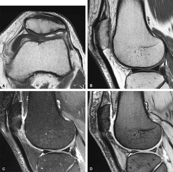
FIGURE 1.1 ● Routine knee examination. (A) Axial T1-weighted 2D fast/turbo spin-echo image. (B) Sagittal proton density-weighted image. (C) Sagittal proton density-weighted image with chemical fat suppression. (D) Gradient-echo image.
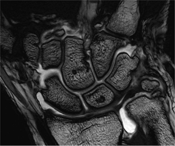
FIGURE 1.2 ● High-resolution wrist arthrography. 3D-FIESTA sequence (steady state free precession), TR 9.2 msec, TE 3.1 msec, voxel size 0.26 × 0.28 × 1.2 mm, acquisition time 3 minutes, 28 seconds.
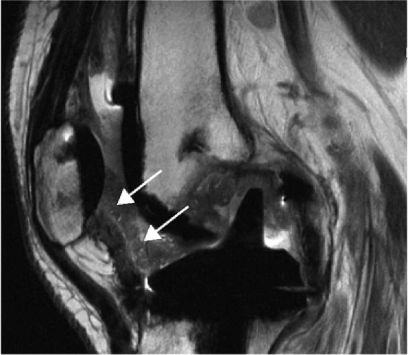
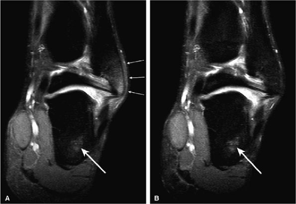
FIGURE 1.3 ● Total knee arthroplasty with synovitis (arrows). Acquired at 1.5 T. Use of an RBW of 83.3 kHz results in limited metallic susceptibility artifact.
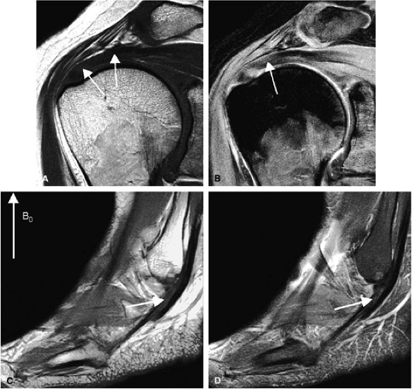
FIGURE 1.4 ● Magic angle effect (arrows). (A, B) Magic angle is seen in a shoulder examination using a short TE (A) and long TE (B). Magic angle in an ankle examination without (C) and with (D) FatSat.
Conventional MR studies are acquired by the serial application of encoding gradients across the field of view (FOV) using a single radiofrequency (RF) coil. The resulting signals received by the RF coil provide data corresponding to the spatial frequency or Fourier components of the object being imaged. Each component of the data, one of a large number of sinusoidal intensity oscillations with specific spatial frequencies, is associated with a particular point in k-space. The central region of k-space, consisting of low-spatial-frequency data, contains information about the gross structure and contrast of an image, most of the information required to produce an MR image. The peripheral portion of k-space, consisting of high-spatial-frequency data, contains information about image detail. Data is usually acquired in a 2D or 3D Cartesian rectangular grid in k-space, moving from one end of k-space to the other, collecting data in sequential parallel lines. An additional line of k-space data in the frequency-encoding direction is serially collected during each acquisition, while sequential lines in the phase-encoding direction are acquired at regular intervals.
Alternative methods of sampling or navigating k-space and of acquiring data are being developed and have the potential to improve both the speed and accuracy of MR musculoskeletal imaging. Two of these techniques, PROPELLER imaging and parallel imaging, are discussed below.
PROPELLER (Radial Acquisition)
Sampling data using the conventional Cartesian technique, with line-by-line sampling of k-space, results in artifacts associated with phase and frequency encoding. Chemical shift results in artifact in the frequency-encoded direction, and motion results in artifact in the phase-encoded direction. Other methods that sample the central and peripheral regions of k-space simultaneously, rather than sequentially in a grid, can reduce these artifacts. Other patterns or trajectories of k-space sampling include radial, spiral, and PROPELLER imaging.
PROPELLER fast spin-echo 1 is a radial k-space filling technique. A range of ultra-low-resolution images are acquired, one per repetition time, with as many phase-encoding steps as echoes in the echo train length (ETL). Each of these scans corresponds to a different rotational direction within the scan plane. Since the data are collected in a series of rectangular strips, serially rotating around central k-space, central k-space is repeatedly sampled. The data set looks like a freeze-frame photograph of a rotating propeller, with the hub located in the center of k-space. Data reconstruction then combines these different data collections in the image domain and corrects or even rejects (based on relative phase information) data acquisitions that are degraded by motion. The resulting final image is relatively free of motion artifact. Also, of particular benefit to musculoskeletal imaging, radial scanning produces fully isotropic in-plane resolution with no frequency and phase direction. Consequently, chemical shift and pulsatile flow artifacts are diffused across the whole image plane, so these artifacts are far less discernible than with Cartesian imaging (Fig. 1.5).
Parallel Imaging
Imaging with a single RF coil, with sequential acquisition of data, point by point, limits the speed with which an MR scan can be performed. Constraints include limits on the amount of soft tissue RF power deposition over a short period of time and limits on the maximal rate of gradient switching of coils. The conventional solutions to these speed limitations, including 1 NEX or fractional NEX imaging and the use of partial phase FOV and shorter repetition times (TRs), have been exhausted. In parallel MR imaging, however, images are acquired with an array of RF coils and the simultaneous acquisition of data over several points, dramatically accelerating imaging times without compromising spatial resolution.2
In parallel imaging, a set or array of RF coils is distributed along the structure to be imaged. The spatial information from this distribution of coils can be used, in addition to spatial encoding from gradients, to generate data for MR image reconstruction (Fig. 1.6). Consequently, fewer gradient steps need be performed and the data set can be undersampled. To maintain spatial resolution, a reduced FOV is used. However, because the data are undersampled in the phase direction, anatomy aliasing or fold-over occurs. Since each of the coils in the array experiences this aliasing differently, based on its coil sensitivity pattern, image reconstruction algorithms, which combine the data from all the coils, can produce an unaliased image similar in appearance to an image acquired from a fully sampled data set. The fold-over signals are “unfolded” using the spatial information from each coil element contributing to the signal in each voxel.
Parallel imaging is capable of scan time reductions, also called “acceleration,” by a factor of 2 to 4 (and experimentally of up to 10). The consequence, however, is a reduction in the signal-to-noise ratio (SNR). The effects on SNR in an

P.5


P.6


accelerated scan (SNR ASSET) are illustrated in the following equation:

in which R is the acceleration factor and g is the geometry factor. The geometry factor is noise, which may be amplified by coil design, the reconstruction algorithm, and certain electromagnetic field fundamentals. An array of coils, optimized for accelerated imaging (ASSET/SENSE), has a g-factor of approximately 1 and does not contribute significantly to the loss in SNR with acceleration. Possible residual aliasing in the phase direction may also degrade image quality.
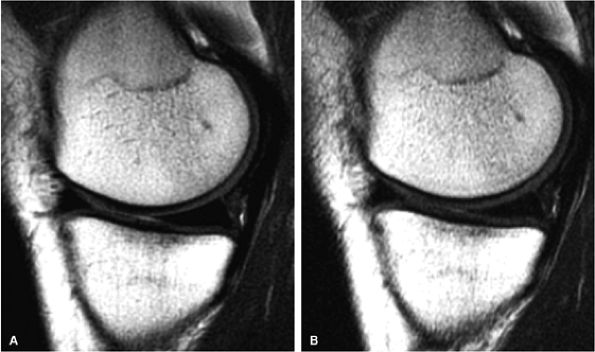
FIGURE 1.5 ● (A) PROPELLER fast spin-echo with a 480 × 480 matrix. (B) Conventional 2D fast spin-echo with 480 × 384 matrix. Scan times were identical. Note an apparent SNR gain in (A) as well as better delineation of cartilage and menisci.
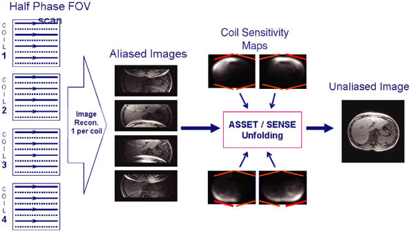
FIGURE 1.6 ● Example of parallel imaging: ASSET/SENSE with acceleration × 2. Half of the raw data are acquired, resulting in half the scan time. SMASH/GRAPPA techniques work in the k-space domain instead of the image domain.
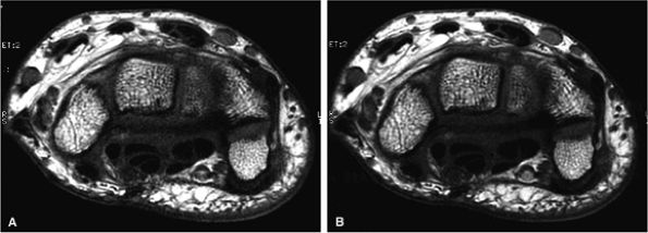
FIGURE 1.7 ● SENSE/ASSET acceleration × 2 with an eight-channel wrist array coil. Axial 2D fast spin-echo (TR 700, TE 16, ETL 2, slice thickness 2 mm, FOV 10 cm, 384 × 320 matrix, 15 slices). With ASSEST × 2 (A), scan time was 58 seconds. Without ASSET (B), scan time was 1 minute 54 seconds. The SNR reduction with ASSET is minimized due to the optimal coil g-factor.
Despite these SNR limitations, parallel imaging can provide improved image quality and spatial resolution using a shortened scan time. For example, wrist imaging is best performed in the difficult-to-maintain “Superman” position, with the surface coil as close to the magnet isocenter as possible. Parallel imaging, with a multichannel coil, can produce a diagnostic wrist study at the rate of 2 minutes per series, or 10 minutes for a complete scan (Fig. 1.7), compared with conventional scan times of 30 minutes.
MR Imaging Protocols
Musculoskeletal imaging protocols were initially dominated by conventional spin-echo and gradient-echo imaging. Conventional spin-echo sequences generate images with excellent soft tissue contrast and perform well in imaging structures with high magnetic susceptibility; however, the sequences are relatively time-consuming. Gradient-echo sequences can dramatically decrease scan times, but some applications, such as echo radial-oblique long axis sequences, which may produce false-positive results in the evaluation of meniscal tears, have proved unreliable. For general peripheral joint imaging, sequences that can be performed quickly (but produce spin echo-like soft tissue contrast) and fat-suppression sequences with sufficient T1 weighting to be sensitive to gadolinium contrast enhancement are essential. For more specific applications, such as cartilage mapping, more complex protocols are needed. A plethora of pulse sequences are currently available, and more are being developed to address these imaging requirements. A few of the more important protocols for musculoskeletal applications are discussed below.
Fast (Turbo) Spin-Echo Imaging
Fast spin-echo sequences produces images similar in appearance and content to conventional spin-echo sequences in a fraction of the time. The advent of spin-echo train acquisition

P.7


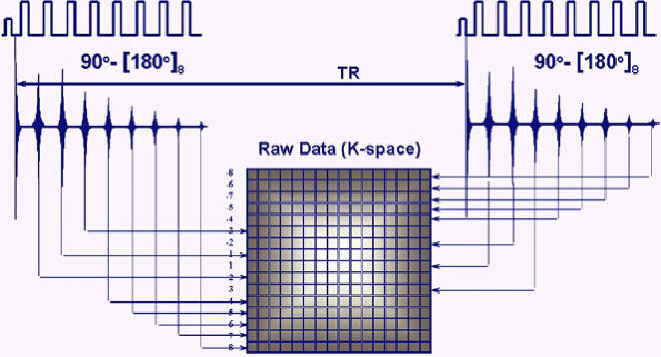
techniques in the early 1990s3 revolutionized MR imaging by allowing the collection of spin-echo data in less time than any of the then currently available gradient-echo or spin-echo sequences. In conventional spin-echo imaging, each echo generates one image. In fast spin-echo imaging, a series of spin echoes, called the echo train, fill lines of k-space, thereby reducing scan time. The series of spin echoes are generated by the use of 180-degree refocusing RF pulses at regular intervals. After each 180-degree pulse, an echo signal is collected that fills a different line of k-space (Fig. 1.8). The images are then reconstructed from the data collected over many echo times (TEs). Scan times are reduced by a factor equal to the number of echoes, the ETL. ETLs vary from 3 to 16. The time between the echoes in the echo train is called the echo train space (ETS) and is generally 4 to 10 msec.

FIGURE 1.8 ● Fast or turbo spin-echo. After each 180-degree refocusing pulse, an echo signal is collected and fills a different k-space line. This accelerates data collection by a factor equal to the ETL.
Signal loss from T2 relaxation occurs progressively during the course of the echo train. The longer the echo train, the more T2 relaxation occurs, with consequent image blurring. In musculoskeletal MR, T2 values range from a few milliseconds for tendons and ligaments to 35 to 40 msec for articular cartilage. As illustrated in Figure 1.9, with application of an echo spacing that is too large and a short TE, only

P.8


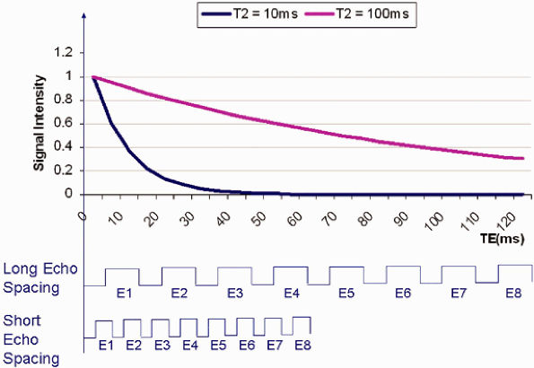
the early echoes of the echo train are seen in structures with a T2 of 10 msec. For tissues with a long T2 (100 msec for instance), all the echoes in the train are seen. The early echoes in the echo train contribute information from central k-space and improve SNR and produce image contrast. The later echoes in the train, with information from peripheral k-space, improve spatial resolution. Consequently, blurring occurs if a long echo train or echo spacing is used for tissues with a short T2 relaxation time, since the raw data from the late echoes that encode high-spatial-frequency details are missing. To minimize blurring when imaging tissues with a short T2 relaxation time, shortening of the ETL and/or the ETS may be required.

FIGURE 1.9 ● Short T2 relaxation times and echo train in fast or turbo spin-echo imaging. If echo spacing is too long, the high spatial resolution is missing from the late echoes, resulting in increased blurring.
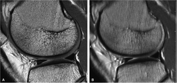
FIGURE 1.10 ● Effect of RBW on fast spin-echo. Note (A) the chemical-shift effect (arrows) on the bone-cartilage interface and (B) the increased blurring due to the longer echo spacing with ± 7 kHz.
Unfortunately, shortening the ETL to improve images of tissues with a short T2 relaxation time adversely affects the potential benefits of reduction in scan times. An alternative solution for decreasing the time needed to perform the echo train, shortening echo spacing, is affected by two other parameters, the frequency matrix size and the receive bandwidth (RBW), both of which control the signal readout time.
Whereas echo spacing changes proportionally with changes in the frequency matrix, it changes inversely with changes in the receive bandwidth. For example, doubling the frequency matrix from 256 to 512 doubles the signal readout time and the echo space. On the other hand, doubling the receive bandwidth from ±16 kHz to ±32 kHz cuts both the readout time and echo spacing in half. Since the frequency matrix must remain as high as possible to achieve the desired spatial resolution, manipulation of the RBW is a critical scan parameter in musculoskeletal imaging (Fig. 1.10).
The RBW affects not only the echo spacing, and secondarily image blurring, but also chemical shift, signal-to-noise, and gradient requirements. The high RBWs that promote short echo spacing result in decreased chemical shift. The chemical shift effect is the frequency shift between fat and water components (220 Hz at 1.5 T), which translates into a spatial shift often visible on images. It can be expressed in number of pixels (Fig. 1.11). However, higher RBWs also decrease signal-to-noise (Fig. 1.12). When the RBW is increased, more noise is collected for the same amount of signal, degrading the SNR. Furthermore, using a very high RBW demands more gradient strength from the system. This may place hardware limitations on the simultaneous manipulation of other parameters, such as FOV and slice thickness, which also make demands on the gradients.
Table 1.1 summarizes the effects of changing RBW and the frequency matrix on image quality. The areas shown in red indicate degradation of image quality; those in green indicate image quality improvement.
TABLE 1.1 ● Effects of Increasing Receiver Bandwidth and Frequency Matrix on Fast Spin-Echo Performance
Fast Spin-Echo Performance Blurring on
Short T2 Species
SNR Spatial
Resolution
Chemical
Shift
Increasing RBW Less Less Unchanged Less
Increasing frequency matrix More Less More Less

P.9


P.10


Fat-Suppression Techniques
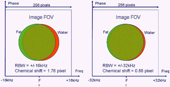
FIGURE 1.11 ● The formula for the chemical shift effect, expressed in number of shifted pixels, is:
For example, with an RBW of ± 16 kHz, the chemical shift is 256 × 220 divided by 32,000, or 1.76 pixel.
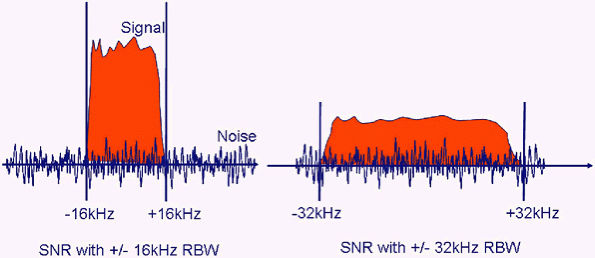
FIGURE 1.12 ● Signal versus noise as a function of the RBW. With ± 32 kHz, the amount of noise that the coil “sees” has doubled, whereas the signal intensity remains the same (red area under curve unchanged).
Diagnostic MR imaging relies on imaging the water content of tissues. Reducing or suppressing the high signal intensity from fat can make these changes in water content easier to discern. Fat signal can be suppressed by several techniques; the STIR, ChemSat or FatSat, and Dixon methods are described below.
STIR Imaging
Historically, the first method for producing fat-suppressed images was inversion recovery, often referred to as short tau inversion recovery (STIR; Fig. 1.13). STIR imaging is based on the differences in the longitudinal relaxation of fat versus water. Fat has a faster relaxation rate or shorter T1 than water. After an initial inversion pulse, images are acquired during T1 recovery when protons from lipids are crossing the null point. Advantages of STIR imaging are that it is relatively unaffected by inhomogeneities in the magnetic field (also called B0) and the radiofrequency field (also called B1). Disadvantages of STIR imaging are its long scan times, relatively fixed TRs and TEs, diminished image contrast, signal loss in tissues other than fat (including those containing water), and insensitivity to gadolinium due to inadequate T1 weighting.
ChemSat or FatSat Imaging
An alternative method for fat suppression is ChemSat or FatSat imaging. FatSat imaging is based on the differences in the precessional frequency of protons in fat versus water. Protons in fat nuclei are surrounded by denser electron clouds than are protons in water nuclei. The electron cloud, in a magnetic field B0, induces an opposing field. Due to this opposing field, the protons in fat nuclei “see” less of the magnetic field than the relatively unshielded protons in water and consequently precess at a lower frequency. Specifically, at 1.5 T, the protons in a lipid molecule (a C–H bond) precess at approximately 220 Hz more slowly than the protons in a water molecule (O–H bond). At 3 T the difference is 440 Hz. When normalized for the field strength, the chemical shift for fat is approximately 3.5 parts per million with respect to water. This difference in precessional frequency can be exploited to suppress signal from fat by applying a presaturation RF pulse to any type of pulse sequence. The spectrally selective presaturation RF pulse is applied in the narrow range of frequencies corresponding to fat, leaving water protons unaffected. The advantages of the ChemSat technique are:
  • Flexibility in image contrast without the TR/TE restrictions characteristic of STIR sequences (Fig. 1.14)
  • Sensitivity to gadolinium
  • Ability to be used with fast gradient-echo techniques with very short TR and TE
The main disadvantage of ChemSat is its sensitivity to inhomogeneity in the magnetic field (B0) and in the RF power distributions (B1), resulting in uneven fat suppression. Incomplete fat saturation is particularly problematic far from isocenter, where the strength and homogeneity of B0 tend to diminish.
FatSat or ChemSat is the most common form of fat-suppression technique currently used in musculoskeletal imaging. Tables 1.2 and 1.3 summarize the respective strengths (blue) and weaknesses (salmon) of STIR and ChemSat techniques.

P.11


P.12


Dixon Method
A third method of fat suppression is the Dixon technique or fat–water separation technique. Similar to FatSat, Dixon imaging is dependent on differences in the precessional frequency of protons in fat versus water. Unlike FatSat, however, which uses spectrally selective pulses to image the frequency shift between fat and water protons, the Dixon method employs nonspectrally selective pulses with TEs that will capture the phase difference between fat and water protons. After the application of a nonselective excitation RF pulse, the transverse magnetization of water and fat are in phase. When in phase, voxel signal is strong since the magnetization is the sum of the fat and water vectors. Over time, due to their differences in precessional rate, the fat and water protons develop a difference in phase. When the phases are at 180 degrees to each other, maximally out of phase, the voxel signal is the weakest due to destructive interference between the water and

P.13


fat magnetization vectors. At 1.5 T, fat precesses at 220 MHz slower than water. At this difference in precessional rate, the time for the phase difference to complete a rotation of 360 degrees is 4.6 msec. Therefore, the TE for in-phase imaging is 4.6 msec or a multiple of 4.6 msec. At this rate, the fat and water vectors will be maximally out of phase, at 180 degrees to each other, at 2.3 msec. Consequently, the TE for out-of-phase imaging is 2.3 msec or a multiple of 2.3 msec. The fat and water in-phase and fat and water out-of-phase images can then be added and subtracted to produce water-only or fat-only fat-suppressed images.

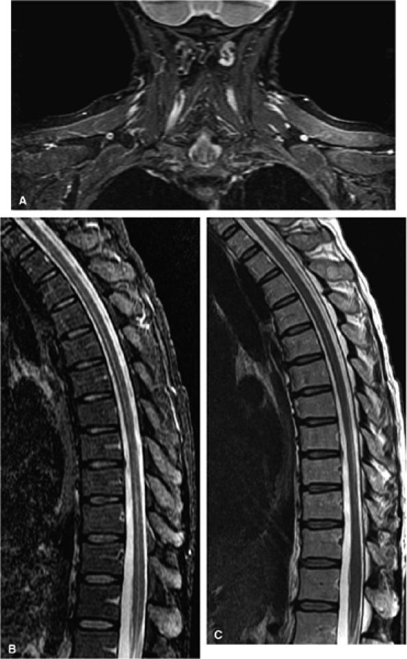
FIGURE 1.13 ● STIR imaging with a large FOV improves image quality in challenging areas such as (A) the brachial plexus and (B) the spine. (C) T2-weighted image for reference. In such applications, chemical fat saturation may show uneven fat suppression.
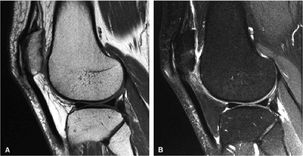
FIGURE 1.14 ● Fast spin-echo proton density-weighted images without (A) and with (B) FatSat. On the FatSat image, fluid and cartilage appear brighter relative to the suppressed fat signal of bone marrow and subcutaneous fat.
TABLE 1.2 ● Comparison of STIR and FatSat Techniques for Fat Suppression, Part I
Fat Suppression
Techniques
B0 Field Strength Robustness Against
B0 Inhomogeneity
Robustness Against
RF Inhomogeneity
STIR Works at all field strengths Very robust Very robust
FatSat Not possible at low field Less robust Less robust
TABLE 1.3 ● Comparison of STIR and FatSat Techniques for Fat Suppression, Part II
Fat Suppression Techniques Image Contrast Gadolinium Sensitivity Scan Time Efficiency
STIR Fixed, proton density T2
(fixed TR/TE)
Very low Long scan time
FatSat All contrasts (any TR/TE) High Very limited time penalty
(fast spin-echo, spin-echo)
The two-point method (one in-phase image and one out-of-phase image) is compromised by sensitivity to magnetic field inhomogeneity. Therefore, a three-point method, collecting one in-phase image and two out-of phase images, is often used. In this method, three scans are performed with different TEs—typically one sequence with a nominal TE value, followed by another with a TE 2.3 msec shorter and a third with a TE 2.3 msec longer. The three corresponding images are analyzed, a phase map is built, and respective water, fat, and combined water and fat images are generated. This technique is termed iterative decomposition of water and fat with echo asymmetric and least-square estimation (IDEAL; Fig. 1.15).
One of the advantages of the Dixon method is that it is relatively insensitive to uneven RF excitation (B1), which result in areas of incomplete fat suppression on FatSat sequences. Since uneven RF field excitation may be caused by complex body shapes (such as are encountered in imaging the brachial plexus, shoulder, hip, ankle, and foot), a sequence that is robust in the face of B1 inhomogeneity is particularly important in musculoskeletal MR applications. Another advantage is its flexibility in the use of a variety of TRs, TEs, and pulse sequences. The Dixon method can be used in spin-echo, fast spin-echo, and 2D and 3D gradient-echo sequences. Disadvantages of the Dixon method include potential blurring in fast spin-echo sequences (due to the extra time required in echo spacing to accommodate the TE variations) and sensitivity to magnetic field (B0) inhomogeneity. This may induce a fat–water reconstruction mismatch, resulting in inversion of entire areas of the image. In addition, certain Dixon techniques are prone to be instable when voxels show a mixed fat–water content, creating reconstruction noise in transitional areas.
Recent developments in acquisition schemes and iterative least-squares reconstruction promise improved robustness of fat–water separation and increased signal-to-noise (Fig. 1.16).4 When image reconstruction times are shortened and multiple image data handling is streamlined, potential applications of Dixon-based solution include imaging of the brachial plexus, shoulder, foot, and ankle, body fat measurements, and bone marrow and growth plate studies.5
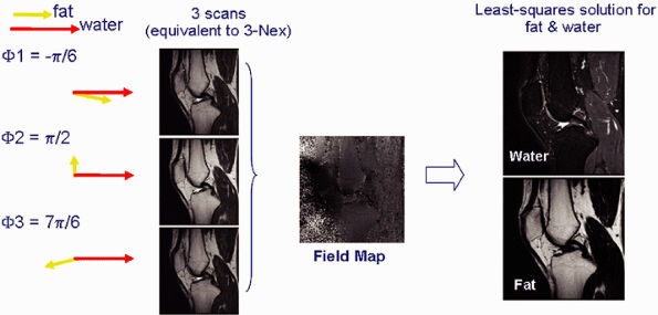
FIGURE 1.15 ● Fat-water separation technique (IDEAL). Images are acquired in three scans with slightly different echo times (and therefore different phase characteristics). The images then undergo phase analysis reconstruction, resulting in images of pure water and fat, as well as a variety of other combinations (such as combined water and fat, in-phase and out-of-phase).

P.14


Metal Artifact Reduction
FIGURE 1.16 ● Comparison of conventional ChemSat (A) with fat-water separation (IDEAL) (B). Note the improved fat suppression in bone marrow, especially in peripheral areas (arrows).
Metal implants and orthopedic prostheses, even when made of nonferromagnetic materials, may cause significant MR artifact, resulting in areas of signal void and image distortion. The source of this artifact is the increased propensity of these materials to become magnetized compared with adjacent soft tissues when placed in a magnetic field. The measure of the propensity of a substance to become magnetized is called magnetic susceptibility. By causing local magnetic field distortion, the magnetic susceptibility of one material may affect not only the magnetic field experienced in the material but also the magnetic field experienced by adjacent materials or soft tissue. These magnetic field distortions result in misregistration artifacts and intravoxel dephasing. Local magnetic field distortion results in misregistration artifact in the frequency-encoding and slice-selective directions due to differential artifactual displacement of signal. The degree of signal displacement or mismapping depends on the intensity of the field strength shifts experienced. Images may be distorted in shape, with areas of signal void with a bright rim. The signal void corresponds to parts of the image that are elongated, and the bright rim is caused by image compression. Local magnetic field distortion results in intravoxel dephasing by causing disparities in the precessional frequency of protons, resulting in phase dispersion. Images may demonstrate areas of partial or complete signal loss (Fig. 1.17A).
The degree of metal artifact is influenced by field strength, and imaging at lower field strengths (such as 1 T) significantly reduce artifact. In addition, positioning the long axis of the prosthesis parallel to the axis of the magnetic field minimizes artifact. Artifact is greatest when the prosthesis is imaged

P.15


perpendicular to the field. The manipulation of several other MR parameters can help to reduce metal artifacts.6 Due to misregistration, metal artifacts are usually greatest in the frequency-encoding direction and are inversely proportional to the frequency-encoding gradient strength. Aligning the frequency-encoding direction along the axis of the metallic implant, increasing the frequency-encoding gradient strength, and increasing the matrix in the frequency-encoding direction all help to decrease the artifact. If the most important images for diagnosis are in the coronal and sagittal planes, frequency-encoding performed in the anterior-posterior direction and phase-encoding in the superior-inferior direction will improve image quality. Increasing the RBW and decreasing the FOV are also critical in minimizing metal artifact (see Fig. 1.17B). Sequence selection is also important. Fast spin-echo images with a long ETL result in less artifact than conventional spin-echo images and much less artifact than gradient-echo sequences. Scans should not be performed with FatSat, since this will accentuate artifacts. Shorter TE sequences result in less artifact. However, TR is not an important variable.

FIGURE 1.17 ● Metal artifact reduction. Coronal fast spin-echo images (TR 3000, TE 44) (A) without a metal artifact reduction technique (ETL 8, RBW 19.2) and (B) with a metal artifact reduction technique including increased RBW and long ETL (ETL 16; RBW 83.3).
Cartilage Mapping Techniques
High-resolution MR cartilage imaging can be achieved by MR techniques that generate parametric cartilage images called T2 and T1 mapping. Imaging is performed with a multichannel phased-array surface coil. In association with high-resolution 3D segmentation for the assessment of cartilage volume and thickness, cartilage mapping may be the first step toward comprehensive, noninvasive cartilage evaluation. These mapping sequences demonstrate subtle signal-intensity changes that are not demonstrated by conventional proton-density and T2 sequences. Research is ongoing into the clinical utility of these techniques in osteoarthritis and other degenerative processes.7 A more comprehensive discussion of cartilage imaging can be found in Chapter 12.

P.16


Cartilage T2 Mapping
T2 mapping is performed using a multi-echo sequence based on fast spin-echo technology. Each echo of the echo train produces a separate image with a different TE (Fig. 1.18). Using a post-processing tool, with a mono-exponential or bi-exponential fit, a T2 value is calculated for each pixel in the image and a color map is displayed (Fig. 1.19).
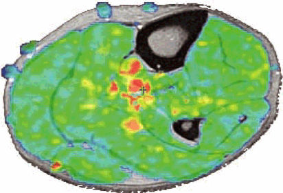
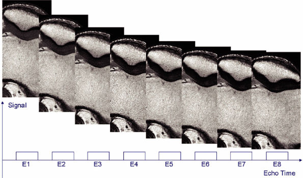
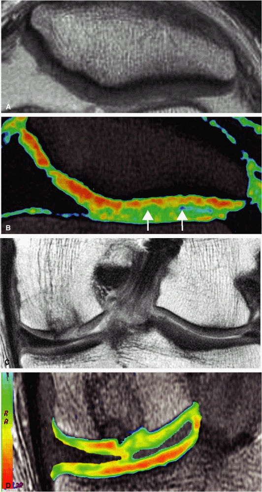
FIGURE 1.18 ● Spin-echo, 8 echoes (10 to 80 msec). Note the signal attenuation in the patellar cartilage. This type of sequence is used to produce cartilage T2 color maps.
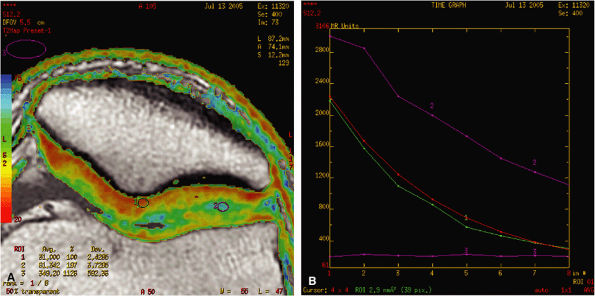
FIGURE 1.19 ● Color map (A) showing T2 values from 20 msec in red to 75 msec in blue, with calculated T2 values from the region of interest (ROI). ROI #1 green curve (B) shows the 8-echo signal pattern, and the red curve shows the calculated monoexponential fit.
Foci of collagen degradation in articular cartilage demonstrate prolongation of T2 values on T2 mapping sequences (Fig. 1.20A, B). Preliminary work indicates a strong correlation between in vivo focal T2 changes and histologic findings. In addition to the assessment of cartilage degeneration, T2 mapping may be useful in the evaluation of autologous cartilage plugs (see Fig. 1.20C, D).
FIGURE 1.20 ● Clinical examples of T2 mapping at 3 T. Color map showing T2 values from 25 msec in red to 75 msec in blue. (A, B) Osteoarthritis (arrow) is not visible on the conventional T2 image (A). (C, D) Autologous osteochondral implant (mosaicplasty) of the medial femoral condyle with mild prolongation of T2 values. (Courtesy H.G. Potter, HSS, NY)

P.17


P.18


There are other sources of cartilage T2 signal variability in cartilage mapping, including normal variations in collagen concentration and collagen fiber orientation. Because of differences in collagen concentration, the surface articular cartilage demonstrates longer T2 relaxation times than those of deep cartilage. Collagen fiber orientation may also affect T2 relaxation times since magic angle artifacts may occur when collagen fibers are at a 55-degree angle relative to the static magnetic field.
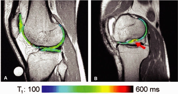
FIGURE 1.21 ● dGEMRIC T1 maps at 1 T. (A) Asymptomatic volunteer (in-plane resolution 450 μ × 450 μ). (B) Patient post-autologous chondrocyte transplantation (in-plane resolution 570 μ × 570 μ). The graft is indicated with an arrow.
Cartilage T1 rho (T1ρ) and dGEMRIC
T1 mapping is performed using a variety of techniques. T1 rho (T1 ρ) images are acquired using multiple 3D gradient-echo scans with various flip angles or spiral look-locker scans. Although they do not take as much imaging time, look-locker scans generate a limited number of slices. For the T1 mapping technique known as delayed gadolinium enhanced MRI of cartilage (dGEMRIC), intravenous gadolinium is administered, followed by physical exercise for 10 minutes and an 80-minute rest period, to promote the extravasation of the contrast material into the joint and uptake in the articular cartilage.
Foci of diminished glycosaminoglycan (GAG) or proteoglycan content demonstrate elevated T1 relaxation on postprocessed T1 rho images. With dGEMRIC T1 mapping sequences, these foci demonstrate decreased T1 after the intravenous administration of gadolinium, indicating a lower GAG level due to increased gadolinium concentration. In healthy tissue, with higher GAG levels, there is less contrast distribution and a longer T1 value. Areas of increased GAG associated with various treatments also demonstrate elevated T1 values (Fig. 1.21).
T1 mapping sequences seem to be complementary to T2 mapping in the assessment of cartilage structural integrity. However, unlike T2 mapping, which is available for clinical applications, T1 techniques are still investigational. Acquisition sequences enabling T1 calculations are technically challenging and not practical, requiring several separate scans. In addition, results of the dGEMRIC protocol are inconsistent due to variability in the performance of pre-scan exercise.
Cartilage Thickness and Volume Measurement
Very recent developments in pulse sequence technology have made possible isotropic high-spatial-resolution 3D imaging, with optimal image contrast. Such sequences permit segmentation of the articular cartilage from the bone and surrounding fluid. The complex shape of the femoral cartilage, similar to a sphere, requires that the imaged voxels have the same dimension in all three directions.
One of the most promising acquisition pulse sequences for isotropic 3D cartilage imaging is fast gradient-echo in steady state (SSFP type), which results in the required contrast. This is coupled with a projection-reconstruction k-space trajectory that results in the necessary voxel isotropy. The sequence, known as VIPR,8 is capable of producing a complete 3D isotropic knee acquisition with 0.4 × 0.4 × 0.4-mm interpolated voxels in just 5 minutes, with a high contrast between cartilage, fluid, and bone, with the advantages of intrinsic fat suppression (Fig. 1.22).
Diffusion-Weighted Imaging and Diffusion Tensor Imaging

P.19


Diffusion-weighted imaging (DWI) produces scans based on proton mobility (or diffusivity). Image contrast is created from intravoxel incoherent motion (IVIM) of water protons.9 Using pulsed magnetic field gradients, the motion of water protons can be demonstrated, and although normally this motion is random, it may be “restricted” in a variety of circumstances. For example, an increase in cell membrane permeability in the setting of stroke results in an influx of water into cells, with a secondary decrease in the volume of the extracellular space. Since the motion of intracellular water is more restricted than the motion of extracellular water, DWI will demonstrate abnormalities in acute stroke much earlier than conventional MR sequences.
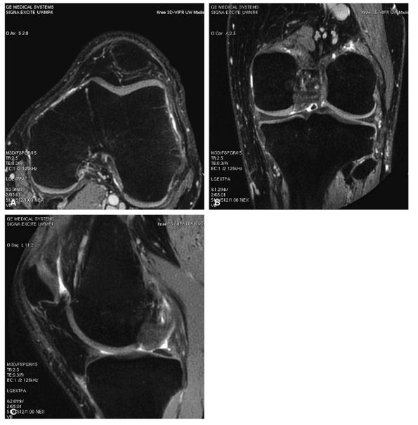
FIGURE 1.22 ● Example of a totally isotropic 3D sequence, 3D-VIPR. Raw data are acquired in a projection-reconstruction mode (not like 2D and 3D Fourier). Reformations (AC) from a unique 3D data set of 0.4 × 0.4 × 0.4 reconstructed voxels, acquired in 5 minutes 1 second. The sequence also provides an intrinsic fat suppression and a T1/T1 image contrast (steady-state free precession). (Work in progress, developed by University of Wisconsin, Madison)
DWI is performed by applying diffusion-weighted gradients during image acquisition. The use of bipolar magnetic field gradients along one of the main gradient axes induces a phase shift for spins moving in that direction, proportional to the spin velocity, whereas stationary spins experience no change in phase (Fig. 1.23). The induced phase shift in the moving spins results in signal attenuation, due to the phase dispersion, directly proportional to the spin velocity. To encode ultra-low velocities (in the range of microns/sec), the sensitization gradients are usually played within a spin-echo echo planar imaging (EPI) sequence, on each side of the refocusing RF pulse, and with a high amplitude and duration. Diffusion scans may be performed at varying degrees of diffusion sensitivity,

P.20


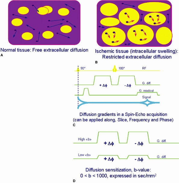
also known as the b-value. The b-value can be increased by increasing the amplitude of the gradients, the duration of the gradient applications, and the time interval between the two gradient pulses. In the images produced, the apparent diffusion coefficients (ADCs) of each voxel can be measured.

FIGURE 1.23 ● Principle of diffusion imaging. (A, B) Biologic tissue shows extracellular fluid random motion (e.g., diffusion) affected by tissue condition. (C, D) By adding specific diffusion sensitization gradients, spins experiencing diffusion result in an attenuated signal due to a net phase shift, unlike stationary spins with no attenuation.
To date, the major applications for DWI have been in neuroimaging, particularly in the diagnosis of acute stroke. However, DWI may also have applications in the evaluation of cartilage. In in vitro experiments, DWI has proved to be sensitive to the detection of early cartilage degeneration.10 Free water in cartilage defects results in regions of visible signal loss compared with healthy cartilage. However, significant impediments exist to the in vivo use of DWI for cartilage imaging, primarily the short T2 relaxation time of cartilage (from 10 msec to 50 msec). The typical diffusion-sensitization gradients in DWI generally increase the TE of EPI-DWI scans to 80 to 100 msec. This long TE results in cartilage signal loss, which limits the application of DWI in cartilage imaging at this time.
As mentioned, in DWI there is an assumption that water molecule motion is potentially random, referred to as isotropic diffusion. However, due to structural characteristics, the potential diffusion may be the same in all three directions, referred

P.21


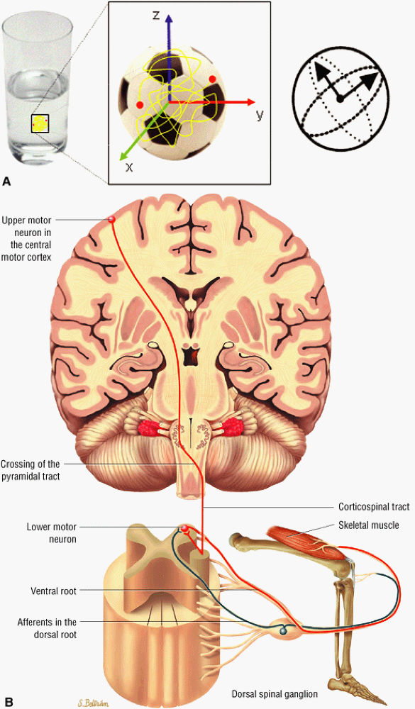
to as anisotropic diffusion. Fiber tracts or myelin sheaths, for example, may limit the direction in which molecules can move. Diffusion tensor imaging (DTI) is a form of DWI that images the directional information of structures such as white matter tracts (Fig. 1.24). Recent advances allow the diffusion data to be processed in color 3D to highlight the trajectories of continuous anisotropy, which are closely correlated with the physical fiber patterns. These direction-encoded color maps, DTI fiber tractography, are depictions of neuronal networks.

FIGURE 1.24 ● Diffusion anisotropy. (A) Free water shows non-oriented diffusion behavior. (B) Posterior view of motor innervation. White matter tracts or muscle fibers show diffusion properties that reflect the orientation or path of the tracts or fibers. In the medulla oblongata corticospinal axons cross the midline in the pyramidal decussation. Ventral roots (motor) reach skeletal muscles through the peripheral nerves.
A potential application for DTI in musculoskeletal imaging is the depiction of longitudinal fiber tract orientation in skeletal muscle. Ongoing studies are exploring the applications of DTI in evaluating neuromuscular degenerative diseases and muscle injury (Fig. 1.25), as well as peripheral nerve pathology.

P.22


P.23


P.24


Advances in Instrumentation
Developments in MR instrumentation are aimed at increasing the speed of scans, improving scan resolution, and producing new MR applications. Advances in surface coil technology permit high-resolution imaging at the FOV requirements of a peripheral joint. Improvements in magnet design have made imaging at higher magnet field strengths practical. Self-shielded 3-T designs have resulted in a fringe field similar to unshielded 1.5-T systems, and short-bore 3-T designs have similar dimensions to 1.5-T magnets. Other developments in 3-T design have reduced the operating cost of a 3-T system by reducing helium consumption and eliminating the need for liquid nitrogen.
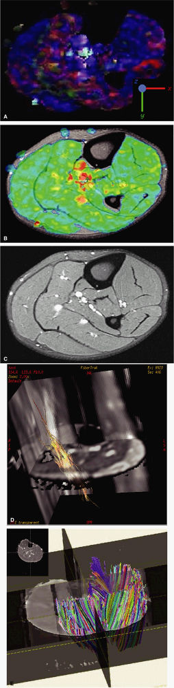
FIGURE 1.25 ● Examples of diffusion tensor MRI in calf muscle. (A) Blue indicates diffusion along the S-I axis. (B) Fractional anisotropy shows the degree of anisotropy regardless of direction. Control image (C) and fiber-tracking display using two different rendering techniques (D, E).
Surface Coils
Dedicated surface coils markedly improve image resolution and are essential in peripheral joint MR (see Chapter 2 for a more comprehensive discussion of surface coils). Small-diameter coils have better signal-to-noise than large-diameter coils, but large-diameter coils have a larger useable FOV. The amount of signal detected after an RF excitation is the same regardless of the size of the surface, but the amount of noise is inversely proportional to coil size. By decreasing the diameter of the surface coil, noise is decreased and the SNR is increased (Fig. 1.26). For example, a small circular loop coil 3 inches (approximately 8 cm) in diameter provides an SNR improvement of 20 to 30 times compared with the body coil. The coil size, however, drastically limits its practical range of use, as its depth penetration is equivalent to its radius (Fig. 1.27).
To achieve the image resolution of a small-diameter coil with the large useable field of view of a large-diameter coil, several small coils can be linked in an array. Phased array coils (Fig. 1.28) use several adjacent receiver coils. Each coil receives RF signals individually but functions with the other coils as an “array.” The system architecture collects the RF signals from each coil on separate parallel chains or “channels” and combines the resulting images into one final image. This magnitude image combination or sum of squares combination affords the coverage possible with a large RF coil and the high SNR possible with a small RF coil.
Until recently, phased-array coils were limited to four RF channels. Compared with a single-channel coil, the single-to-noise gain is on the order of 30% to 50% (Fig. 1.29). The next generation of phased-array coils have eight or more coil elements. The first musculoskeletal eight-channel coil was designed for the knee. Compared with the single-channel birdcage extremity coil design, the eight-channel knee coil delivers at least 20% more SNR at the center and up to 100% more SNR near the periphery (Fig. 1.30).
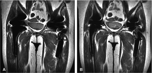
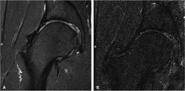
FIGURE 1.26 ● Hip examination, coronal fast spin-echo proton density-weighted image with FatSat (TR 3100, TE 41). (A) Images acquired with a four-channel cardiac array coil. (B) Images acquired with a body coil. The signal-to-noise improvement with the array coil is at least 100%.

P.25


P.26


P.27


3-T Imaging
3-T imaging has rapidly become accepted as the next phase in high-field MR imaging. Imaging at higher field strengths improves SNR (Fig. 1.31), resulting in higher-resolution imaging and decreased scan times. The relationship between SNR and magnetic field strength, although complex, is almost linear between 0.5 T and 3 T. The SNR at 3 T is approximately twice that at 1.5 T (Fig. 1.32). In addition, fat suppression is more robust at 3 T than 1.5 T.
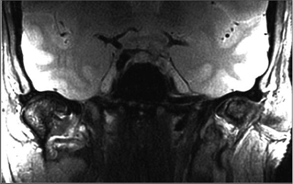
FIGURE 1.27 ● Bilateral temporomandibular joint study, with two circular 3-inch coils. Note the strong signal attenuation from outside to inside. As a rule, the optimal depth zone for a circular coil is equal to its radius-that is, about 1.5 inches (4 cm) from the coil inner surface.
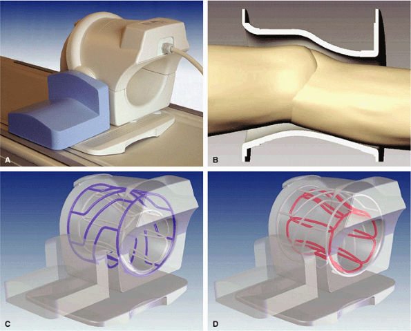
FIGURE 1.28 ● Phased-array knee coil. (A) Split-top design. (B) Coil tapered to the knee shape to maximize SNR and patient comfort. Coil is made of an RF transmit birdcage (C) and eight longitudinal RF loops for reception (D).
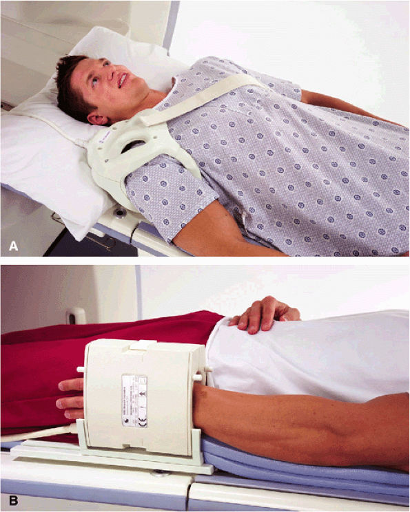
FIGURE 1.29 ● Examples of dedicated musculo-skeletal RF coils. (A) Three-channel shoulder (the shoulder array coil is available in four- and eight-channel designs) array coil; note the underarm RF loop. (B) Four-channel (the eight-channel wrist array coil is also used in the neutral wrist position) wrist array coil. This coil can also be used in the horizontal position, closer to the magnet isocenter, with the patient prone and with the arm extended above the head (the “Superman” position). This less-comfortable position is sometimes required when the system does not deliver good image quality with widely off-centered coil positions.
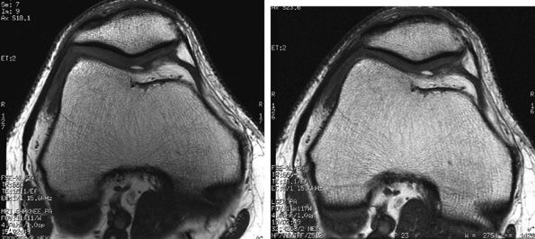
FIGURE 1.30 ● Image quality improvement with an eight-channel knee array coil (A) compared to a four-channel extremity coil (B). Note the increased SNR in the patellofemoral cartilage area.
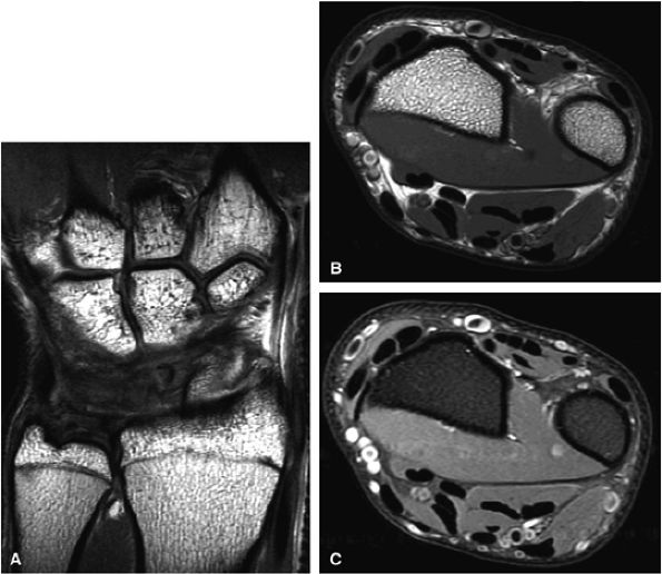
FIGURE 1.31 ● 3-T imaging of the wrist. Coronal proton density-weighted image (A) and axial proton density (B) and proton density fat-suppressed (C) images of the wrist.
Scanning at 3 T requires some adaptations. Because power deposition increases as the square of the field strength through 5 T, the risk of RF patient heating is markedly increased at 3 T, requiring specific absorption rate (SAR) management. The TR may need to be increased to permit heat dissipation and smaller flip angles are required in RF-intensive sequences like fast spin-echo, which are near maximum SAR guidelines at 1.5 T. Although SNR is improved, image appearance at high field is slightly different. T1 and to a lesser extent T2 relaxation times are prolonged. T1 relaxation times increase by up to 30% at 3 T compared with 1.5 T. Chemical-shift artifact doubles, necessitating the use of higher RBW protocols. Similarly, susceptibility artifacts, like those from metal surgical implants, are stronger. In large FOV acquisitions, such as body imaging, spatial variation in the B1 field may cause image artifacts. The B1 is highest at the skin, decreases with increasing

P.28


depth, and then increases centrally. This variation in B1 may result in image edge and center brightening. For most musculoskeletal applications, however, the potential benefits with higher-resolution imaging and improved fat suppression are substantial.11

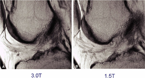
FIGURE 1.32 ● Sagittal proton density-weighted images of the knee acquired with identical parameters at 3 T and 1.5 T. Note the improved SNR of the 3 T image (A) versus the 1.5-T image (B).
References
1. Forbes KP, Pipe JG, Karis JP, et al. Improved image quality and detection of acute cerebral infarction with PROPELLER diffusion-weighted MR imaging. Radiology 2002;225:551-555.
2. Pruessmann KP. Parallel imaging at high field strength: synergies and joint potential. Top Magn Reson Imaging 2004;15:237-244.
3. Melki P, Mulkern RV, Dacher JN, et al. [Fast spin echo MRI techniques. Contrast characteristics and clinical potentials]. J Radiol 1993;74:179-190.
4. Reeder SB, Pelc NJ, Alley MT, et al. Rapid MR imaging of articular cartilage with steady-state free precession and multipoint fat-water separation. AJR Am J Roentgenol 2003;180:357-362.
5. Donnelly LF, O—Brien KJ, Dardzinski BJ, et al. Using a phantom to compare MR techniques for determining the ratio of intraabdominal to subcutaneous adipose tissue. AJR Am J Roentgenol 2003;180:993-998.
6. Petersilge CA, Lewin JS, Duerk JL, et al. Optimizing imaging parameters for MR evaluation of the spine with titanium pedicle screws. AJR Am J Roentgenol 1996;166:1213-1218.
7. Gray ML, Burstein D, Xia Y. Biochemical (and functional) imaging of articular cartilage. Semin Musculoskelet Radiol 2001;5:329-343.
8. Gu T, Korosec FR, Block WF, et al. PC VIPR: a high-speed 3D phase-contrast method for flow quantification and high-resolution angiography. AJNR Am J Neuroradiol 2005;26:743-749.
9. Le Bihan D, Turner R, MacFall JR. Effects of intravoxel incoherent motions (IVIM) in steady-state free precession (SSFP) imaging: application to molecular diffusion imaging. Magn Reson Med 1989;10:324-337.
10. Miller KL, Hargreaves BA, Gold GE, et al. Steady-state diffusion-weighted imaging of in vivo knee cartilage. Magn Reson Med 2004;51:394-398.
11. Kornaat PR, Reeder SB, Koo S, et al. MR imaging of articular cartilage at 1.5T and 3.0T: comparison of SPGR and SSFP sequences. Osteoarthritis Cartilage 2005;13:338-344.


This website uses cookies to improve your experience. We'll assume you're ok with this, but you can opt-out if you wish. Accept Read More