
– JOINT RECONSTRUCTION, ARTHRITIS, AND ARTHROPLASTY > General >
CHAPTER 100 – DESIGN AND PERFORMANCE OF JOINT REPLACEMENTS
Director of Biomedical Engineering, Cooper Union Research Foundation,
Albert Nerken School of Engineering, 51 Astor Place, New York, NY 10003.
was interposition arthroplasty using soft and flexible materials, but
the strength of these materials was inadequate. Rigid materials such as
metal and glass in the form of condylar shapes attached to one of the
joint surfaces provided some success, but there was still a problem
with the apposing joint surface. In the knee, geometric inaccuracy
leading to poor kinematics and abnormal soft-tissue tensions was also a
problem. An interesting finding with condylar components, such as cup
arthroplasty or MacIntosh tibial plateaus, was the formation of a
fibrous membrane adjacent to the component, with a new bone plate
beneath. This tissue modeling is now recognized to develop due to
interface micromotion and to the stresses acting on the exposed
trabecular ends. Even now, implants are designed with relatively smooth
surfaces interfacing the bone; however, there is a higher incidence of
pain, migration, and loosening with these implants compared with the
more rigid methods of fixation. The success of more invasive components
with uncemented intramedullary stems, such as hemiarthroplasties and
knee hinges, depended largely on obtaining an acceptably low level of
stem–bone micromotion and interface stresses on the bone (33).
when Charnley introduced cemented metal-polyethylene components for the
hip, and in the late 1960s, when this technology was transferred to the
knee by Gunston (95). The principles proposed
by Charnley were rigid fixation of the components to the bone,
resurfacing of both joint surfaces, and the use of materials with low
friction and wear. These principles, embodied in cemented
metal-on-plastic components, have stood the test of time to this day (100,112).
of total joints used. A number of other hip designs were introduced
that were fundamentally based on the Charnley design. An exception was
the use of metal-on-metal in the McKee-Farrar design. There was a great
deal of attention to surgical technique, especially obtaining good
cement–bone apposition with high shear strength. Some total knees
proved to be successful in the long term, but others fell by the
wayside because of the lack of recognition of the kinematics, the role
of the cruciates, the patellofemoral mechanics, and the requirements
for adequate fixation. Most of the design forms used today, namely
unicompartmentals, condylar replacements with or without cruciate
retention, mobile bearing knees, stabilized condylars, and fixed and
rotating hinges, were all introduced before the end of the decade.
Ceramic-on-polyethylene and ceramic-on-ceramic replacements for the hip
had been introduced before 1980.
sophisticated instrumentation, especially for the knee, and uncemented
components with porous coatings intended for indefinite fixation. In
the knee, improved consistency of surgical technique was achieved as a
result of more accurate alignment and soft-tissue balancing. Concerning
porous coating, those designs in which rigid initial fixation was
achieved obtained sufficient bone ingrowth for long-lasting results.
Certain uncemented designs of hip stem, acetabular component, and
femoral component of the knee have shown survivorship values (54) superior to those of cemented components. A hydroxyapatite (HA) coating (104,203)
has similarly shown high durability from 5 to 10 years follow-up. The
situation today is that a number of designs of hips, knees, and other
joints have been shown to have a survivorship of greater than 90% at 10
years, such that the large majority of elderly patients can be treated
confidently. Today’s hip and knee systems offer a large variety of
sizes and modular augments to deal with virtually every situation
encountered in primary and revision surgery. The instrumentation
systems are elaborate, usually well engineered, and often too complex,
but they allow the surgeon to achieve accurate component placement and
limb alignment.
are excessive wear of the ultra-high molecular weight polyethylene
(UHMWPE) (126,236) and
loosening. These two problems are related to some extent in that the
accumulation of small particles causes a tissue response that, in turn,
produces bone resorption. However, it is now evident that wear can be
reduced in a number of ways. The main problem has been that
gamma-irradiation of UHMWPE in air, followed by gradual oxidation
either on the shelf or in the patient, has led to a degradation of
mechanical properties and an increase in the wear rate (18,140,180).
have shown a reduced susceptibility to oxidation, which has resulted in
reduced surface wear and a much lower incidence of the destructive
delamination seen in total knee replacements (TKRs) (27).
Gamma-irradiation and storage in an inert atmosphere, as well as
enhanced cross-linking and stabilization to minimize subsequent
oxidation, have resulted in reduced wear rates. For the hip joint,
ceramic-on-UHMWPE can reduce wear by as much as 50%, whereas
ceramic-on-ceramic and metal-on-metal produce minimal wear debris (65,82).
If such improved bearings are combined with superior cement techniques
or porous and bioactive coatings, much greater durability can be
expected compared with that achieved in the past 2 decades.
subsurface stresses is still a threat. Computer modeling of this
process has now shown how appropriate surface geometry can
substantially reduce the likelihood of delamination without
compromising the freedom of motion (189). New
advances will undoubtedly be made in the performance of TKR, especially
for younger patients. The mobile bearing concept is one such approach
for minimizing wear and improving function. However, further advances
are likely in the form of guided motion knees providing optimal muscle
lever arms and high flexion ranges. The superior functional performance
of unicompartmental replacement performed on one or both sides of the
joint opens up the possibilities of minimally invasive surgery (84),
with the option of using computer-assisted technologies. The boundary
between biologic treatments and total joints will become an issue, and
with both approaches improving and developing, the relative merits and
applications will become an area for extensive research and evaluation (59,70,72,79,141,142,152,162,165,177).
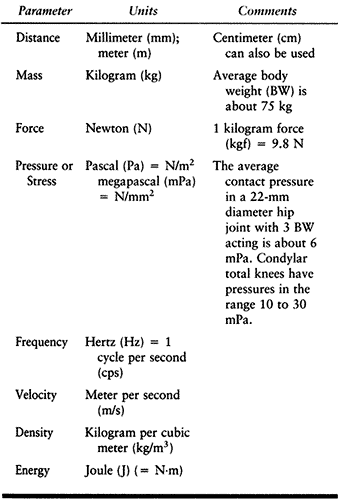
concepts of biomechanics and biomaterials relevant to joint replacement (159). The Standard International (SI) system of units (Table 100.1) is now in widespread use.
 |
|
Table 100.1. SI System of Units
|
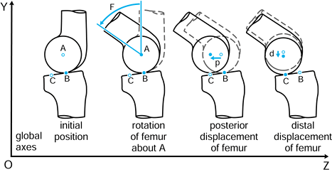
p in the negative Z direction. Finally, the femur is given an
additional displacement d along the negative Y direction. The tibia has
remained fixed with respect to the global axes, and the femoral motions
could be described with respect to an axis system fixed in the tibia.
The values F, p, and d are vectors in that they have magnitude and direction, often denoted with a line above or in bold type.
 |
|
Figure 100.1.
Motion in a plane. Global axes, axes in the femur, and axes in the tibia are defined. In this case, three successive motions of the femoral axes relative to the global axes are shown: F, p, and d. |
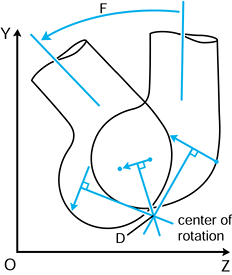
not to be confused with the geometric centers of local radii of
curvature. If the instant center is at the center of curvature, the
motion at the contact point is called pure sliding (124). If the center is at the contact point, the motion is pure rolling (31). A center in between the two produces sliding and rolling combined.
 |
|
Figure 100.2. Any two successive positions of a body in a plane can be obtained by a rotation about a single point.
|
define rotations and displacements with respect to axes, rather than
using centers of rotation (238) by the following principles:
-
Define a global axis system.
-
Define axes in each bone.
-
Define each component of motion of one axis system relative to the other.
-
Define the order in which the motions take place.
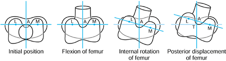
the femur is shown in its initial position on the tibia at zero flexion
with contact points L and M. The femur is first rotated by 90° (flexed)
about a transverse axis through A. Next the femur is rotated about a
vertical axis through A fixed relative to the tibial axes. The lateral
contact point moves posteriorly by a and the medial anteriorly by a. The femur is next translated posteriorly by a. The lateral contact point has now displaced posteriorly by a total of 2a,
but the medial condyle is in its original position. In orthopaedic
terms, as the knee has flexed, there has been an internal rotation of
the tibia and a posterior translation of the femur.
 |
|
Figure 100.3.
Three-dimensional knee motion described by successive rotations and displacements. The figure depicts “average” knee motion from the extended to the flexed position. |
posterior displacement of the lateral contact point can occur on an
unrotated or rotated tibia, producing a slightly different end result.
The entire motion could have been achieved by a single rotation about
and a displacement along a screw axis (235),
but this is more difficult to visualize conceptually than the sequence
of rotations and displacements described. In addition, the internal
rotation and posterior displacement could have been achieved by a
rotation about a vertical axis through the medial tibial condyle.
Hence, it is important to define the method of describing the motion
and which axes are used, to avoid misunderstanding and confusion.
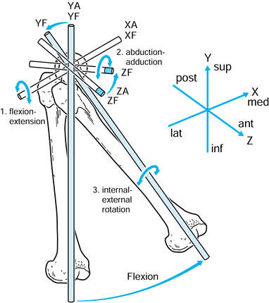
of the femoral head and the vertical axis is through the center of the
knee (Fig. 100.4). The anteroposterior (AP) and
mediolateral (ML) axes are self-evident, and all axes are mutually
perpendicular. The axes in the acetabulum and femur are conveniently
defined as being coincident with the hip in the neutral position. The
motion of the femur is defined in relation to a fixed acetabulum as
follows:
 |
|
Figure 100.4. Axes in the hip joint.
|
-
Flexion-extension about the XA axis.
-
Abduction-adduction about the ZA axis.
-
Internal-external rotation about the YF axis.
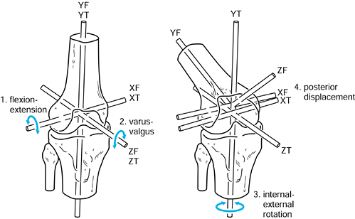
The transverse axis in the femur can be chosen through the epicondyles.
The other two axes are mutually perpendicular. For convenience, the
axes of the tibia in the initial reference position at zero flexion can
be taken to be the same as for the femur. Ordered motions are defined
for the femoral axis system relative to the tibial axis system.
 |
|
Figure 100.5.
Axes in the femur and tibia used to describe successive rotations and displacements. Flexion of the femur about XT, varus about ZT, external rotation about YT, and posterior displacement along negative ZT are shown. |
-
Flexion-extension about XT.
-
Varus-valgus about ZT.
-
Internal-external rotation about YT (this can also be regarded as rotation of the tibia about YT).
-
AP displacement along ZT.
used to define a set of order-independent motions of the knee. This is
the Grood-Suntay system (93), which has the advantage of ease of visualization.
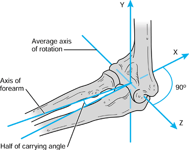
it is useful to define the axes with respect to the axis of rotation,
rather than using the long axes of the bones. The description of the
motion can then be simplified to a single degree of freedom by the
choice of the axis, which
bisects the carrying angle (Fig. 100.6).
This axis becomes a common axis in the humerus and ulna, the other two
axes being mutually perpendicular as shown. In this case, the long axes
of the bones are not coincident with the reference axes.
 |
|
Figure 100.6.
For a uniaxial joint such as the elbow, one of the axes in each bone is taken along the axis of rotation, which bisects the “carrying angle.”. |
different motions and the paths from the initial position to the final
position. Successive rotations about three axes as shown in the
preceding figures are called eulerian or cardan angles (6,235). Transformation matrices
consisting of sines and cosines are used to convert the coordinates of
points on the object from the initial to the final position with
respect to one of the defined axis systems. A major interest in
artificial joints is the continuum of motion during dynamic activities,
an aspect that will be discussed later.
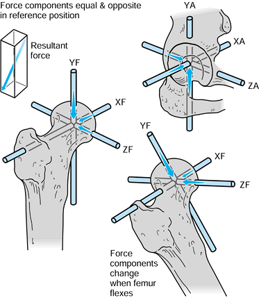
case, they have magnitude, line of action, and point of application.
Exactly the same axis systems used for the bones can be used to define
the forces. For the hip in the neutral position, there are three components of force along each of the three axes, which can be combined into a single resultant force (Fig. 100.7). The forces on the femoral head are exactly equal and opposite
to those on the acetabulum. If the femur is now moved to any arbitrary
position, the resultant forces on the femoral head and in the
acetabulum will still be equal and opposite. However, the three
components of force along each of the femoral axes are now different
from those along the acetabular axes. Hence, when defining the forces
across a joint, it is important to specify the axis system to which the
forces are referred. In reality, of course, the resultant force is
representative of the pressure acting over a large surface area.
 |
|
Figure 100.7.
When the axes in the femur and acetabulum are coincident, the three components and the resultant are equal. When the femur moves, the resultant is the same, but the components along the femoral axes are different. |
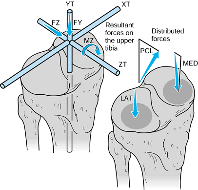
to the upper tibia. The compressive force and the varus moment produce
a larger resultant force on the medial condyle than on the lateral
condyle. The forces themselves are representative of the contact
pressures and act at the center of pressure
of each contact area. The shear force is transmitted to the tibia by
the contact areas being on the upward anterior slopes of the tibial
plateaus and by a force in the posterior cruciate ligament (PCL).
 |
|
Figure 100.8.
Forces and moments acting on the upper tibia with respect to axes. The forces are shown distributed to the condylar surfaces and to the posterior cruciate ligament. |
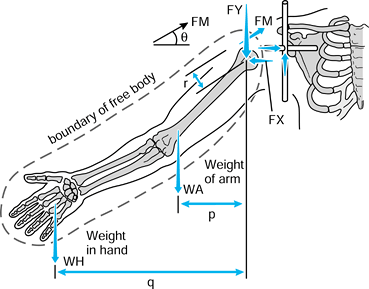
in which the problem is to calculate the forces on the face of the glenoid with the arm abducted and a weight in the hand (174). The steps are:
 |
|
Figure 100.9.
To calculate the unknown forces at the joint, the forces are drawn and the arm is isolated as a “free body,” shown by the dotted line. |
-
Define axes in each bone. The humeral
axes are not drawn here because only the forces with respect to the
glenoid are considered. -
Define the forces on the glenoid. In this example, only the forces in the scapular plane FY and FX are considered.
-
Draw these forces equal and opposite on the humeral head.
-
Draw the other forces on the arm, namely the muscle forces FM, and the external forces WA (weight of the arm) and WH (weight in the hand).
-
Define the arm as a free body by drawing a boundary around it and showing the forces that act across the boundary.
radiographs), there are three unknowns, namely FX, FY, and FM. Three
equations are thus required to obtain a solution.
humeral head, so their moments are zero.) The individual values are
then solved from these three equations. This concept of isolating a
defined entity as a free body
and analyzing the forces across the boundary can be applied to numerous
force analysis problems in the body. As with motion, the changing
pattern of forces during activities is important.
depicted with lines of action, in reality the forces are transmitted
across areas on the joint surfaces. This results in a contact pressure, or contact stress, acting on the surface (124). The density of the subchondral bone plate will provide an indication of the pressure distribution (161).
are used. Whereas static analysis, as shown in the previous section,
can be used to calculate resultant forces, to calculate pressures and
stresses in an implant-bone system, more complex analyses are required.
For simple geometries, elasticity (e.g., hertzian) equations can be
used to calculate the contact areas and stresses in terms of the radii
and the elastic properties of the materials. However, for realistic
bone and implant shapes, finite element analysis (FEA) (15,16,44,175) is the most appropriate technique.
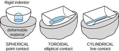
is hemispherical, with the maximum pressure at the center being 1.5
times the mean pressure. The same situation occurs if the lower surface
is flat, a convex spherical surface, or a concave spherical surface.
 |
|
Figure 100.10. Three types of contact in joints: spherical, cylindrical, and toroidal.
|
-
Higher force.
-
Lower elastic modulus (stiffness) of the materials.
-
More conforming surfaces.
-
Longer time the force is acting (due to “creep,” defined later).
-
Higher force.
-
Higher elastic modulus.
-
Less conforming surfaces.
-
For a stiff layer under a relatively soft layer.
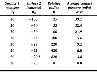
curvature for the two surfaces, and the radius of curvature is taken as
positive for convex surfaces and negative for concave surfaces.
on a flat surface. The average contact pressures calculated for a given
force (1000 N) and material properties (metal-on-plastic) are shown in Table 100.2. This table shows how the relative radius and the contact
pressure change dramatically as the surfaces approach full conformity.
The range covers a nonconforming knee to a hip joint with a small
femoral–acetabular clearance (15). Note, however, that the standard hertzian equations lose accuracy when the contact radius (R2) approaches the surface radius (R1). Another factor is that the contact pressure does not necessarily predict the wear rate, which is so often assumed (148).
 |
|
Table
100.2. The Relative Radii of Curvature and the Contact Pressure in a Spherical Metal-Plastic Contact, Covering the Range from Knees to Hips, for a Compressive Force of 1000 Newtons |
curvature) has a much larger contact area than does a sphere on the
same flat surface (Fig. 100.10). Examples of
arthroplasties with such contacts include some knees, elbows, ankles,
and fingers. Today, most geometries in condylar knees are toroidal,
between spherical and cylindrical, producing elliptical contact areas.
This has the advantages of reducing contact stresses and avoiding
“digging-in” at the sides if tilting occurs. The stresses beneath the
surface in all types of contacts are extremely important in both
natural and artificial joints, in terms of producing subsurface damage.
(Note that the word “stress” can be substituted for the word “pressure”
in this context.) In the case of metallic cemented or uncemented hips,
the contact pressures are highest in the proximal-medial region but
with high pressures distal-lateral also. The magnitudes of the
pressures depend also on stem geometry and head offset. For uncemented
stems, in which a “perfect” metal–bone fit is not achieved, local
contact pressures can be very high due to the stiffnesses of the
materials. An additional interface effect is due to friction between
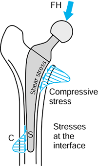
the metal and the bone, causing shear forces to act as shown in Figure 100.11 (101,198).
If there is bonding across the interface from cement or from a porous
or HA coating, the shear forces will be higher, decreasing the
interface contact pressures. The interface shear stress is defined as:
 |
|
Figure 100.11.
Interface contact pressures and shear stresses for intramedullary fixation of a hip. The magnitudes of these stresses vary considerably depending on stem design, fixation method, bone geometry, head offset, and other factors. |
-
Positive contact pressures at those interfaces that usually experience compression (e.g., acetabulum, upper tibia).
-
Minimum contact stresses on interfaces that usually do not experience compression (e.g., intramedullary canal).
-
Minimum shear stresses (e.g., acetabulum, upper tibia, intramedullary canal).
avoid intramedullary fixation, or to design the component to minimize
tension and shear.
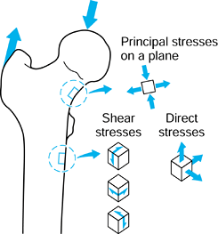
forces are acting, in general, there will be stresses acting in the
plane of the surface (Fig. 100.12). If a small square is drawn on the surface, there will be one direct stress (tensile or compressive) acting on opposite faces and another direct stress acting on the other pair of faces. There will be a single value of shear stress
acting to distort the square. If the square is now rotated, an
orientation can be found at which the shear stress is zero. The direct
stresses acting at this orientation are called the principal stresses.
One of these is the maximum and the other the minimum. Tension is taken
to be positive; compression negative. However, the principal stresses
can be both negative, both positive, or one negative and one positive,
depending on
the loading conditions around the square of surface. The maximum shear stress is at 45° to the principal stresses.
 |
|
Figure 100.12.
At a location on a surface, there are two direct stresses and two shear stresses. An orientation can be found at which the shear stresses are zero. The direct stresses are now the principal stresses. A similar situation applies to a three-dimensional element of material. |
same. Here, a small cube of material is taken, which has three direct
stresses and three shear stresses. At a certain orientation, the shear
stresses are zero and the direct stresses are again called the
principal stresses.
This term is convenient in that it describes the stress state at a
point with a single number. In fact, it is calculated from the three
principal stresses, and is a value that quantifies the likelihood of
yielding, synonymous with the yield stress in direct tension.
which is the amount of energy (force × distance) stored in the material
due to the applied stresses deforming the material. This quantity is
considered to be relevant to bone remodeling, whereby the response of
osteoblasts within the bone material is proportionate to the amount of
deformation and hence strain energy density. This is an “elastic”
quantity recoverable on removal of the stresses, but yielding of the
material is an additional consideration.
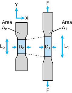
and not to the shape of the object, whether it be a bone or an implant
component. A fundamental property is modulus of elasticity E, which can be determined by a simple tensile or compressive test on a cylinder (Fig. 100.13):
 |
|
Figure 100.13. A simple tensile test to calculate the modulus of elasticity E.
|
strain is small, usually measured in microstrain. A typical strain
value for the cortex of a long bone under peak load is on the order of
2000 to 3000 microstrain. For materials such as cartilage and ligament,
however, the strain can be 10% or more, and hence the true stress after load application must be related to the deformed area σT = F/A1, where A1 is the area with the force applied. Poissons ratio ν defines the strain in directions perpendicular to the longitudinal strain:
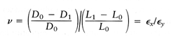
0.4, and for an incompressible material such as a fluid or rubber, ν
equals 0.5.
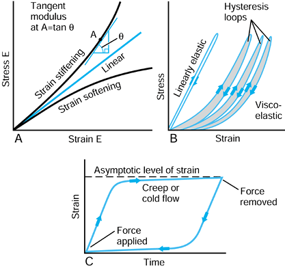
but increases steadily with strain. Rubbers usually exhibit strain
stiffening also. Conversely, materials such as polyethylene exhibit
strain-softening behavior, in which the elastic modulus appears to
reduce with strain. For these nonlinear materials, modulus of
elasticity has to be defined as a tangent modulus at a particular value of strain, as shown in Figure 100.14A.
 |
|
Figure 100.14. A: Metals usually have a linear stress-strain curve. Biologic materials, rubbers, plastics, and composites are usually nonlinear. B:
An elastic material recovers its initial shape immediately on load removal. For a viscoelastic material, there is a residual displacement and a hysteresis loop. C: Characteristics of creep or cold flow, when the load is maintained over a period of time, and then removed. |
is an immediate strain, followed by a continued strain at a decreasing
rate, reaching an asymptotic level (Fig. 100.14C). The behavior is called creep or cold flow.
When the force is removed, the reverse process occurs. Polyethylene
behaves in this way, as does articular cartilage, tendon, and ligament.
Stretching exercises before a sporting activity put such tissues
through viscoelastic and creep cycles. Acrylic cement, when subjected
to sustained loading in a fluid environment at 37°C, shows some creep,
and this may be relevant to the slight sinkage of polished hip stems
over time.
if a property such as modulus or strength is much greater in only one
particular direction. Most biologic materials are orthotropic, which
results from their structure, either aligned collagen fibers in the
case of ligament and tendon, or aligned osteons in the case of bone (128).
Articular cartilage is a special case with complex properties due to
its triphasic composition of collagen fibers, mucopolysaccharide
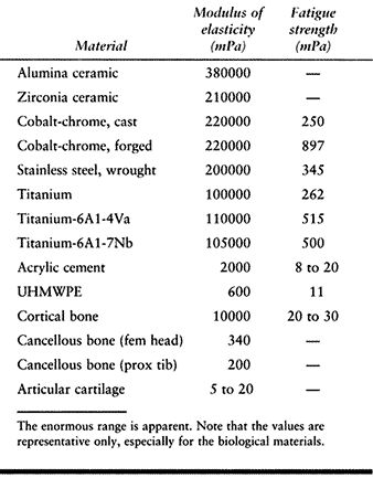
matrix, and fluid. The values of modulus of elasticity for the
materials discussed cover a wide range (Table 100.3),
and consequently, the transfer of forces between different structures
is complex and can involve regions of stress concentration.
 |
|
Table 100.3. The Modulus of Elasticity and the Fatigue Strength of Biological and Artificial Materials
|
either tension, compression, or shear. In general, tensile failure is
the most common. If a material is stretched and fails suddenly, that is
termed brittle fracture. Ceramics and acrylic cement behave in this way. Metals and polyethylene, on the other hand, are ductile in that there is a region of plastic deformation whereby the material elongates at essentially the same applied load. If the load is released, there is a permanent deformation,
but the material can continue to be structurally useful in that
condition. Permanent deformation in plastic tibial and patellar
components is an example. Tendons and ligaments behave as if they were
numerous fascicles in combination (41,241),
with rupture of the tightest fascicles occurring first. If the load is
released and sufficient fibers are intact, the structure can still
function. Bone is close to being brittle, although there is some
plastic deformation due to pull-out of osteons from the matrix (58,128,159).
the level at which single cycle yield or fracture occurs due to
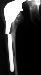
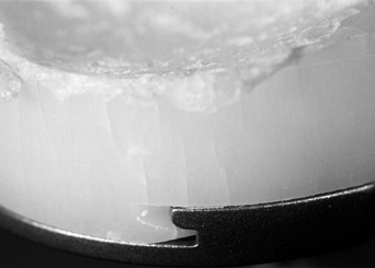
repetitive cycling of forces, a process known as fatigue. This process has been observed on many orthopaedic devices including hip stems (93) (Fig. 100.15), tibial trays (1), and plastic liners (Fig. 100.16). The fatigue strength or fatigue limit is the stress below which no failure would occur no matter how many cycles of loading occurred (Table 100.3).
This value is generally about two thirds of the failure stress for a
single-load application. Fatigue failure initiates at the location of
the highest stresses, and the crack gradually propagates through the
section until the stress reaches the level at which complete failure
occurs at a single load. The starting point of the crack can be a small
defect in the material structure, such as an intergranular defect in
metal or plastic (205). Even a reference
number of a component etched onto a metal surface in a highly stressed
region has been the initial location of a fatigue crack. Such defects
are called stress concentrations or stress raisers in that they raise the stress level above the overall average level in that region (106).
Sharp edges, corners, or grooves in implant components are common sites
of stress concentration. Even defects just within the material, such as
small bubbles in cement, can act as stress concentrations in the same
way. Generally, biologic materials do not experience fatigue failure
because the resting periods between loading episodes allow for
restoration and remodeling. However, one theory for the development of
osteoarthritis has been advanced: healed trabecular microfractures,
failed in fatigue, produce an overly stiff supporting structure to the
articular cartilage.
 |
|
Figure 100.15.
A fractured revision hip stem, in which the lower part of the stem is rigidly supported but the proximal region was relatively unsupported, especially medially. |
 |
|
Figure 100.16.
Fatigue cracks in an UHMWPE tibial component. This is due to a degradation of mechanical properties from oxidation in a component that had been on the shelf for several years. |
change rapidly from section to section, especially in the presence of
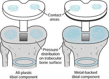
implants. Combinations of bone and implant are called composite structures. An example of a component that acts in series with the bone is a metal-backed tibial plateau (Fig. 100.17).
It is assumed that the resultant forces on the plastic surfaces are
similar for the all-plastic and metal-backed components. However, at
the resection level of the upper tibia, although the forces transmitted
across this section are the same, the distribution is quite different.
In the case of the plastic, there are high stresses directly under the
contact areas. In contrast, the metal plate spreads the load over the
entire upper tibia. The actual pressure distribution largely reflects
the foundation stiffness of the underlying trabecular bone (154). At an individual trabecular level, the stresses are largely compressive in a vertical direction in the normal knee, but are
varied and complex beneath an artificial knee, depending on the
penetration and closeness of contact of the cement. At the level of the
cortex, below the implant level, the stresses in the prosthetic case
are similar to those of the normal knee.
 |
|
Figure 100.17.
The stress distribution on the upper tibial surface depends on whether the component is all-plastic or metal-backed. In the latter case, the distribution reflects the foundation stiffness of the trabecular bone. In the cortex, the stresses are equal and resemble normal. |
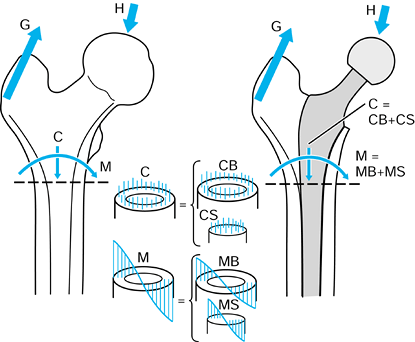
These two stress distributions are combined to produce the resultant
stresses. The bending stresses usually dominate over direct stresses
such that the lateral side is still in tension and the medial side is
in increased compression.
 |
|
Figure 100.18.
The stresses in the bone at a section just below the lesser trochanter, for the intact femur, and after insertion of a hip stem. See text for details. |
is called the bending stiffness. In practice, a hip stem has a much
higher EI value than the bone for a narrow cortical thickness and large
canal diameter. In this case, the proportion of the bending carried by
the stem is high, and the bone can be seriously stress protected. At the other extreme, with a thick cortex and a narrow canal, the bone carries a high proportion of the bending.
Human joints are different from most bearings in engineering in that
they operate under low sliding speeds and are expected to last a
lifetime. Furthermore, they are constructed of a thin soft layer on a
relatively hard layer, carry out motions in multiple directions, and
are not necessarily fully conforming. The way in which they function so
effectively is in maintaining a layer of viscous fluid between the
cartilage surfaces such that direct rubbing of cartilage on cartilage
occurs infrequently (227). A number of
different lubrication mechanisms known in engineering have been found
to apply to human joints, but their behavior is so complex that there
is no direct analogy. The coefficient of friction,
defined as the ratio of the frictional shear force to the compressive
force, ranges from about 0.001 to 0.01. This means that, for a typical
compressive force of 3 body weight (BW) (2000 N) on a hip or knee, the
shear force is a mere 10 N. In contrast, a metal-polyethylene joint
would have a shear force of at least 10 times that. Although friction
is usually associated with sliding between two surfaces, a frictional
shear force can also be transmitted during rolling, up to the level
determined by the dynamic friction coefficient. The motion in that case is termed tractive rolling.
During a lightly loaded swing phase, synovial fluid is drawn in between
the joint surfaces. On applying a force at the start of stance, a fluid
film is maintained by a squeeze film
mechanism, whereby the large surface area and the viscosity of the
fluid mean that leakage of the film occurs at a very low rate. As
movement begins, the film is further maintained or even enhanced by elastohydrodynamic lubrication,
by which the area of contact is maintained due to the deformations of
the bearing surfaces and fluid is pressurized as it is drawn into a
thin converging wedge between the surfaces. In addition, as the
cartilage surfaces are deformed, fluid is exuded between the surfaces
(this has been termed weeping lubrication)
and at the leading edge of the contact area. Fluid becomes trapped in
small undulations in the cartilage surfaces, a mechanism called trapped pool lubrication, and a higher concentration of
hyaluronic acid can result in a more viscous layer of synovial fluid, by so-called boosted lubrication.
The hyaluronic acid protein complex chemically binds to the cartilage
surface so that even if sliding occurs when there is minimal film
thickness, boundary lubrication is provided.
lubrication mechanisms are ineffective because of the hardness of the
materials and the limited surface areas, so that surface-to-surface
rubbing takes place during sliding. At each step, it is estimated that
millions of submicron-sized plastic particles are released into the
joint. The effect of wear on particles and osteolysis of the bone
around the interface, as well as the mechanical effects of the change
in geometry, are major limiting factors in the durability of artificial
joints (82).
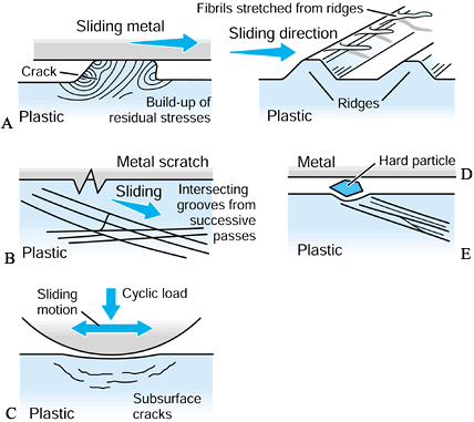
visualized as the sticking of a tiny region of the plastic surface on
to the metal surface such that a fragment of plastic is pulled away (Fig. 100.19). It is now thought that such a mechanism may require multiple passes to build up sufficient strain energy in the asperity
(a local high point) before it is released. A variation of this
mechanism occurs when the adhesion results in a small fibril of plastic
being stretched from an asperity and eventually released. The next
mechanism is abrasive wear (83). In two-body abrasive wear,
small sharp asperities on the metal surface, such as scratches, cut
into the plastic surface. Crisscrossing of scratches on the plastic due
to variations in motion paths accelerate this type of wear. Three-body abrasive wear occurs due to the entrapment of small particles between the sliding surfaces (51).
In artificial joints, these particles can be plastic, acrylic cement,
bone, HA, or metal debris from rough or sprayed surfaces. If such
particles embed into the plastic surface, they can accelerate the wear
locally. All of these mechanisms produce particles in the range of 0.1
µm to a few microns. The particle shapes are granules, fibrils, or flakes (47,48).
For ceramic-on-ceramic or metal-on-metal joints, the wear mechanisms
are similar but the rates of volumetric wear are much smaller than for
metal-on-polyethylene joints, and the particle sizes are also smaller.
 |
|
Figure 100.19. A representation of different wear and damage mechanisms from a plastic surface: adhesive wear (A), two-body abrasive wear (B), three-body abrasive wear (C), delamination (D), and fretting (E).
|
This is a fatigue process whereby shear stresses at about 1 mm beneath
the surface change in direction as sliding and rolling take place,
initiating and propagating cracks in the material (176).
When the cracks reach the surface, fragments of plastic are liberated.
A surface once disrupted fragments at a rapid rate. It is noted that,
because delamination is affected by subsurface stresses, it can occur
due to rolling as well as sliding, although the stress magnitudes are
slightly higher in sliding. Pitting is
another fatigue damage phenomenon caused by tensile cracks initiating
at the surface. The effect is usually local, seen as pits about 0.5 to
1.0 mm in diameter. The severity of both delamination and pitting
depend on the fatigue properties of the material, which, in turn, may
depend on time-dependent phenomena such as oxidative degradation (62,77,135,180,182).
-
The material properties change (e.g., due to yield, surface heating, in vivo oxidation, chemical effects).
-
The surface of an initially polished hard material becomes scratched.
-
Transfer films occur (e.g., due to surface heating, degraded joint fluid).
This occurs due to cyclic shear stresses across an interface between
two parts intended to be statically fixed together. Examples are a
modular femoral head on a taper and a plastic insert in a metal
backing. The shear stresses can be generated due to elastic
deformations from cyclic loading, including the Poissons effect. The
latter occurs, for example, when the plastic of
a
tibial component becomes squeezed radially outward from a contact area.
The motion due to the interface shear stresses can be submicron or even
up to a millimeter in a loose snap-fit connection.
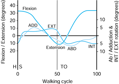
On heel-strike, there is about 30° of flexion, and at toe-off, about
10° of extension. The other two rotations are approximate because of
the difficulty of separating femoral from pelvic motion. However, the
range of abduction to adduction is about 11°, and for internal-external
rotation, the range is about 8°. These rotations produce motions of
individual points on the femoral head that traverse curved paths in the
socket and cross over one another. This aspect is discussed further in
the section dealing with hip-simulating machines.
 |
|
Figure 100.20.
Representative values for the rotations occurring in the hip joint during normal walking. (Data from Inman VT, Ralston HJ, Todd F, eds. Human Walking. Baltimore: Williams & Wilkins, 1981.). |
determined indirectly by using gait analysis and directly in total
joints by using telemetry (20,21,187).
The latter is more applicable to the subject of this chapter. These
forces have been depicted as acting on the femoral head during
different activities. Figure 100.21 shows that
the line of action of the force during level walking changes much less
than the angles of motion of the femur relative to the acetabulum. The
projection on the acetabelum of these forces during walking results in
a similar pattern but with larger angles of excursion. This means that
the force vector moves somewhat more with the femur than it does with
the acetabulum (74,75). The reason for this is that approximately two thirds of the hip force is produced by the abductors (10), which tend to apply their force parallel to the long axis of the femur (74,75).
 |
|
Figure 100.21.
The magnitudes and directions of the forces on the femoral head during the stance phases of different activities. (The data were determined by using telemetry [21].) |
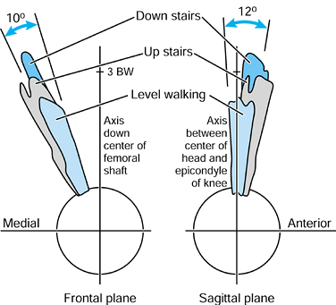
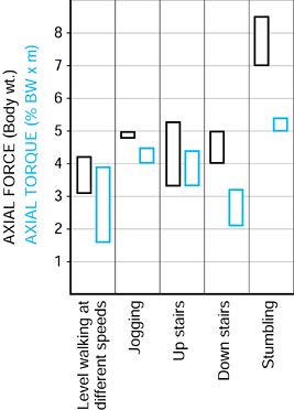
important to the function of total hips. For this purpose, it is useful
to consider the forces relative to axes based on the long axis of the
femur. In the frontal plane, the force makes an angle of 15° to 27° to
the long axis of the femur during stance. This produces axial
compression, a varus moment, and a medial-to-lateral force. In the
sagittal plane, there is an important component peaking at
approximately 0.75 BW acting from an anterior to posterior direction on
the femoral head, which results in torsion (21,99).
The latter is considered to be an important contributor to the
compressive failure of trabecular bone in uncemented stems, and results
in stem fractures initiating from an antero-lateral corner.
The exceedingly high force of 8 BW encountered accidentally in a
stumble is important because a single force such as this, along with
its torsional component (21), could lead to debonding at the implant–bone, cement–bone or cement–stem interfaces, or to cracking of the cement mantle (22,150,210). A factor that influences the mechanics of the hip is the offset of the femoral head from the femoral axis (167,184).
This is frequently reduced from normal in a total hip replacement
(THR). The effect is an increase in the force required in the abductors
(10), leading to a higher resultant joint
force, a more vertical resultant, and sometimes a gait abnormality. An
increase in offset reduces forces but causes an increase in the bending
moment on the stem. Failure to achieve the
normal anteversion of the head and neck increases the axial torsion, which is undesirable (21).
 |
|
Figure 100.22.
The ranges of the peak forces in different activities measured by telemetry in two different subjects. (Data from Bergmann G, Graichen F, Rohlmann A. Hip joint loading during walking and running, measured in two patients. J Biomech 1993;26:969.) |
little since the original Charnley design, although paradoxically, even
a small change in design can result in a major change in performance.
Fundamentally, the stem shape parallels the canal shape (167),
leaving space for a cement mantle of 2 to 4 mm in thickness. In early
designs such as the Charnley, Exeter, Stanmore, Muüller, and T28, the
cement was not intended to bond to the stem. In contrast, at the
cement–bone interface, these designs aimed for an intimate mechanical
contact with rough bone or trabecular bone. Compressive, shear, and
tensile stresses are transmitted to the bone surface (113), an unnatural situation, but one that is tolerated for long time periods.
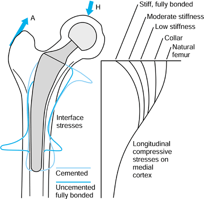
changed from normal due to the presence of the stem, especially
proximomedially, where the longitudinal compressive stresses are
reduced to 20% to 30% of normal levels (110,223) (Fig. 100.23).
Progressing distally, the stresses become closer to normal, reaching
normal levels below the level of the stem tip. The reduction in a
stress parameter, such as the Von Mises stress, particularly when it
results in a reduction of bone density or volume, is called stress protection or stress shielding (30).
Over a time period of approximately 5 to 10 years, this results in
longitudinal removal of bone at the neck cut level, osteopenia, and
resorption of bone away from the cement. If this process becomes
extreme, the interface stresses around the remaining stem become
excessive (150), leading to “clinical” loosening (94).
In addition, wear particles can be more easily transported down the
interface, producing lysis at locations all around the stem, especially
distally (98). A further consequence of
proximal bone loss is that the stem is only rigidly fixed in its distal
half, increasing the bending stresses and increasing the possibility of
fatigue fracture (94).
 |
|
Figure 100.23.
Typical direct (compressive and tensile) stresses at the bone interface, and the longitudinal compressive stresses in the bone, after cemented or uncemented stems. The proximomedial stress-shielding is least with a functional collar and most with a fully bonded stiff stem. Some data are adapted from various papers by R. Huiskes and colleagues (see, e.g., references 113,114). |
become the standard method for measuring and monitoring changes in bone
density over time (201,202).
In this technique, in the frontal plane, for example, an x-ray beam is
scanned across the field, and measures of x-ray absorption are made,
giving a measure of bone mass at a matrix of points in the field. Major
changes in bone mass usually occur slowly, and it has been found that
bone loss may be only 10% to 20% at 2 years, but that this loss can
increase to as much as 50% in the proximal-medial region at 5 years.
known only approximately, but the goal is to minimize these stresses
and to avoid local stress concentrations. Stresses within the bone
should be as close to normal as
possible.
Cement and stem stresses, especially tensile, should be minimized and
should not exceed the fatigue limit under normal loading conditions.
All of these goals cannot be obtained simultaneously, but a number of
guidelines for hip stem design exist:
-
Stem bending stiffness should be much lower than that of the bone to minimize stress shielding.
-
Avoid excessively flexible stems that elevate interface tensile and compressive stresses and produce excessive micromotion.
-
Ensure that the cement mantle thickness is a minimum of 2 to 3 mm (122) (can be achieved using centralizers).
-
avoid corners or any other feature on the stem that would cause stress concentrations in the cement or in the stem itself (22).
-
Create smooth contours but with sectional shapes that will not twist within the cement mantle.
-
Provide features such as proximolateral
projections (e.g., “cobra” design) to provide a greater connection
between stem and cement, a net increase in compressive stresses, and a
reduction in tensile stresses -
Provide a means of centralization,
especially proximomedial and distal, to avoid close metal–bone
proximity, where lysis frequently occurs. -
Use third-generation cementing
techniques, including cleaning the canal, distal plugging,
pressurizing, and minimizing porosity (12,145)
long-term clinical data suggest that a smooth surface or a near-smooth
surface, in which there is no direct stem–cement bonding, produces
successful results. The use of rough surfaces, or rough surfaces with a
precoating of cement to obtain stem–cement bonding, has not been
uniformly successful. It appears that shear and tensile stresses at the
interface can cause progressive debonding and interface micromotion (150).
The latter can then generate metal and cement debris, which enter the
joint space, followed by accelerated wear of the UHMWPE liner. Evidence
of stem–cement micromotion in all types of stem is frequently seen in
retrievals and produces fretting wear of both stem and cement (Fig. 100.24).
 |
|
Figure 100.24.
A retrieved hip stem showing that the original matte surface has been polished smooth due to micromotion between the stem and the cement. This is due to fretting wear. |
and forged cobalt-chrome or stainless steel is usually preferred.
Titanium alloys have been prone to surface wear or even crevice
corrosion and are not in general suitable for cemented application. The
ideal combination for a cemented stem with a modular head is to use
cobalt-chrome alloy for both owing to the minimal corrosion on the
taper connection (31) and reduced scratching of
the femoral head over time. Other head materials are discussed later in
this chapter. Because of its success in elderly patients, and even in
younger patients (12,71,145)
(although studies are variable on this issue), it is unlikely that the
design of the standard cemented stem for primary cases will change
substantially in the foreseeable future. Long-stem cemented components
are used in revisions, but the cement penetration and shear strength
are likely to be inadequate owing to the loss of most of the cancellous
bone from the previous implant (146).
solid UHMWPE hemisphere, or just greater than a hemisphere, with
grooves on the outer surface for keying to the cement. A metal wire is
usually embedded on the outside to measure the wear relative to the
femoral head on radiographs. The range of motion (ROM) between the
femoral neck and the socket before impingement occurs is important
because it affects the potential for dislocation as well as loosening.
It is notable that, as wear proceeds, the ROM steadily reduces, and
this process can lead to problems for 22 mm heads in the long term. The
factors affecting ROM are:
-
ROM increases with head diameter. (However, there is an increase in volumetric wear with diameter.)
-
ROM increases with decreasing neck
diameter. (This is especially applicable to flexion-extension, in which
the neck can be elliptical.) -
ROM decreases with a short neck if collar-socket impingement occurs.
-
ROM decreases with “skirted” femoral heads, which increase head height and offset.
-
ROM decreases in certain planes if the socket and stem are malpositioned.
diameter in the range of 26 to 28 mm with an elliptical neck of minimum
diameter for strength. In practice, the most widely used diameters are
28 mm and 22 mm. To obtain sufficient plastic thickness the minimum
outer diameters of the acetabular component recommended for a 28 mm
diameter head are 44 mm for plastic and 48 mm for metal-backed plastic.
Below those diameters, a 22 mm head is recommended.
are the same as those for stems, notably intimate contact of the cement
with a rough bone surface and penetration within the trabeculae. There
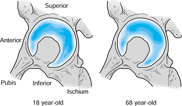
is still uncertainty regarding removal of the subchondral plate (161) and the size and number of key holes (Fig. 100.25).
Although retention of a subchondral plate is attractive for force
transmission, areas of relatively smooth bone are prone to interface
micromotion, bone resorption, and particle ingress. The loosening
mechanism of cemented acetabular components is that the peripheral
regions become infiltrated with UHMWPE debris, leading to bone
resorption, followed by a creeping process that eventually involves the
entire interface (192). This process has been
conceptualized as a progressive increase in the “effective joint
space.” Mechanical factors are also likely to play a role due to higher
than normal stresses occurring in the trabecular bone (64).
Steady migration of sockets into the acetabular bone is common, and
acetabular component failure usually occurs at a higher rate than for
stems in follow-up examinations after more than 10 years. The use of
metal backing (115), which reduces the
incidence of interface radiolucency in tibial components, has not been
successful in cemented acetabular components. Simple finite element
models indicated a more uniform stress distribution across the
interface, but more complex 3-D models, which included the exact
shapes, bone densities, and forces acting (64),
have shown otherwise. This has highlighted the care needed in
formulating and interpreting finite element models and the conclusions
that may be drawn from them.
 |
|
Figure 100.25.
Density of the subchondral bone in the acetabulum for two different ages. Assuming that the density reflects load transmission, in youth (left), there is more even distribution, which gradually converts to more localized superolateral load transmission over time (right). (Data from Muüller-Gerbl M. The Subchondral Bone Plate, Vol 141. Advances in Anatomy, Embryology and Cell Biology. Berlin: Springer-Verlag, 1998.) |
hemispherical shells were interposed between reamed surfaces of the
femoral head and acetabulum in the expectation that new cartilaginous
surfaces would form between the metal and the bone. The tissue
formation, however, was unpredictable, consisting of localized islands
of fibrocartilage and hyaline articular cartilage. There may still be
possibilities for this type of approach if the type of tissue formation
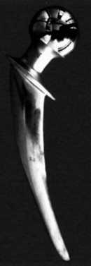
can be controlled to a greater degree. The Austin-Moore and similar
hemiarthroplasties, generally with rectangular sectioned stems, were
moderately successful with regard to fixation and pain relief, although
most of the patients had limited functional requirements. Subsequently,
many such uncemented stems with “satin” or smooth interface surfaces
have been introduced in total hip stems, but have all been subject to
bone resorption, interface micromotion, and migration, leading to
unsatisfactory results.
achieving tolerable stresses at the implant–bone interface and
minimizing interface micromotion to approximately 50 µm or less over
most of the interface. These conditions depend on the surface of the
stem, the sectional shape, and the overall geometry. The major factors
are
-
Stem Surface.
Smooth or satin stem surfaces are unsatisfactory and become surrounded
by a thin layer of fibrous tissue and a bony shell, which is linked to
the cortices with trabecular struts. Rough surfaces have been
successfully used in designs such as the Zweymuller (PLUS,
Endoprothetik AG, Switzerland) in cases in which rigid mechanical
fixation with the diaphysis has been achieved at surgery. In suitable
stem designs, porous surfaces have shown at least 25% of the surface
area ingrown by bone, which has proved to be adequate for long-term
fixation (42,80). The rate of bone ingrowth and the percentage of area ingrown are enhanced with HA or HA-tri-calcium phosphate (TCP) coating (203).
Such coatings superimposed on rough or macrogrooved surfaces have
demonstrated enhanced bone growth around the periphery of the stem, but
bone
P.2590
has been sparse when gaps have been greater than approximately 1 mm (90,203).
In all of the above-mentioned cases, the strongest bone attachment and
areas of new bone formation have been where the implant was in contact
with cortical bone or strong cancellous bone, in regions where high
forces are transmitted (42,80,194). -
Stem Sectional Shape (Fig. 100.26).
Circular or elliptical sections have the least potential for bone
attachment, except where an initial interference fit is achieved and
the stem is rough or coated. Corners that cut into the bone have been
successful, but again only for certain surfaces and where the overall
stem geometry has avoided excessive stresses at the stem corners.
Grooves cut into the stem provide little benefit unless they are
provided with a bioactive coating such as HA. On the other hand,
multiple cutting flutes, especially when combined with a rough surface,
provide stable fixation, particularly in torsion (232). A useful application of such flutes is in revision stem design (131)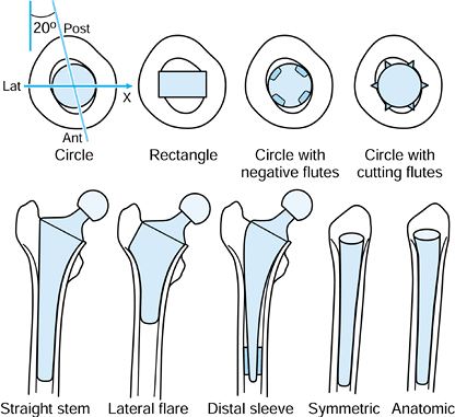 Figure 100.26.
The shape and orientation of the normal diaphyseal canal is shown. The
most rigid fixation of stems occurs when the corners of a rectangular
stem or longitudinal cutting flutes cut into the cortical bone.
Osseointegrated straight stems provide rigid fixation at the expense of
proximomedial stress-shielding and difficulty of removal. The lateral
flare provides rigid fixation and allows for a shorter stem, especially
when designed anatomically in the ML view. -
Overall Stem Geometry. In the frontal view, most stems are either straight or have a lateral flare (Fig. 100.26).
Generally, it has been found that reliable long-term fixation is
obtained when rigid initial fixation has been achieved and most of the
stem is rough or coated to promote subsequent bone apposition or
ingrowth. Two examples are the Zweymuller and the AML (DePuy, Inc.,
Warsaw, IN). The main disadvantage of this approach, especially when
the stem is both porous coated and long, occurs when removal of an
ingrown stem becomes necessary. The lateral flare designs with a high
neck cut attempt to maximize proximal fit-and-fill such that the stem
can be of reduced length. This is possible because the proximal shape
reduces the bending moment on the stem and also provides rigid axial
load support. The stems are usually anatomic in shape, as seen in the
ML view, to maximize the proximal fill. A question with uncemented
stems is the number of sizes needed to provide adequate fit both
proximally and distally in the large majority of cases. Some designs
address this by using modular distal sleeves (50).
Collars are an effective way of increasing the compressive stress
component in the proximal femur, but this can be achieved reliably only
if there is osseointegration into the underside of the collar (57,71).
more proximal stress shielding than a cemented stem owing to its larger
cross-sectional area (38,80).
Laboratory tests have shown that this is not necessarily the case
because the stem becomes tightly wedged in the femur, producing high
circumferential tensile stresses as well as up to 50% of the axial
compressive stress component (226). Where
proximal bone ingrowth has been achieved, bone has been well preserved
over time, based on DEXA-scanning data. However, serious proximal bone
loss has occurred under the following conditions:
-
Rigid distal fixation and inadequate proximal fixation.
-
High bending stiffness of stem compared with bone (80) (i.e., thick stem, thin cortex)
-
Excessive stem length.
revisions. The major goals in the design of a revision stem are to
maximize axial and torsional stability, and to preserve or enhance the
remaining bone. To achieve these goals, the following features are an
advantage:
-
A stem with distal longitudinal cutting
flutes and a bone attachment surface (e.g., rough or HA-coated) to
provide torsional, axial, and bending stability; if necessary, the long
stem inserting into the diaphysis past the level of the previous stem. -
A proximally filling stem with cutting fins and grooves, and a bone attachment surface to attach to and load the proximal bone.
-
A lateral flare to enhance axial stability, increase proximal bone loading, and reduce the bending moments on the distal stem
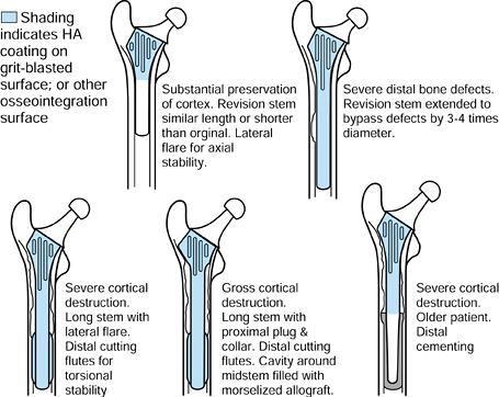
as well as patient factors, a graduated implant system is logical,
basing the design decision on a hierarchy of factors (Fig. 100.27).
Modular systems using separate proximal “plugs” and distal stems, or
using a hollow proximal sleeve with a stem that locks within it (as in
the S-ROM [DePuy-J&J, Warsaw, IN] system) (45)
are useful approaches in dealing with these variations in an
off-the-shelf system. A fragile or detached greater trochanter is
problematic and can be held by hooks or wires. Circumferential bone
wiring reduces hoop stresses on surgical insertion but may cause stress
concentrations in future years. The most difficult revision situation
occurs when the diaphysis below the level of the failed stem is thin.
Here, the choice is between impaction allografting (91),
with a risk of migration, or a very long uncemented or cemented stem
affixing in the femoral condyles. The long stem can even be rigidly
attached to a knee replacement in those cases in which both the hip and
knee need revising or replacing.
 |
|
Figure 100.27.
A graduated approach for a revision hip system in which various design features are added according to the condition of the femur and status of the patient. |
made for providing a custom hip for every case, provided the surgery is
suitably precise (14). For a cemented hip,
there must theoretically be an ideal thickness and shape of cement
mantle and an ideal stem length. For an uncemented hip, there must be
an ideal fit and stem length to minimize interface micromotion (109) and produce the ideal combination of interface and bone stresses (110,232).
In all cases, the ideal position of the femoral head can be obtained.
However, the issue is complex, and separate considerations apply to
cemented or uncemented, primary or revision (49,131). Some of the factors that are noted in the argument against the widespread adoption of custom stems are as follows:
-
The stem design itself is only one part
of the total operative procedure. Larger variations in clinical results
may occur owing to technique variables rather than owing to the stem
design. This point includes the fact that custom stems are not
necessarily positioned in the intended location in the femur. However,
a “Robodoc” type of approach (computer-controlled milling of the
femoral canal based on preoperative computed tomographic [CT] imaging)
might provide the eventual answer to this problem (14,171). -
Long-term deterioration of fixation, such
as interface bone resorption and “clinical loosening,” may be dominated
by biologic factors at the interface, including the effect of wear
debris. -
There are no validated theoretical models
for determining the ideal shape for a hip stem for any particular
femoral geometry. Hence, the nearest fit from an off-the-shelf system
may be as favorable as a custom design if the latter is designed by
nonvalidated rules. -
Achieving an accurate fit-and-fill of a
stem to the cortical bone (or an exactly uniform cement mantle) may not
produce the ideal conditions for long-term success (181).
This has been demonstrated for a closely fitting stem, but one without
a surface that provided osseointegration, such as porous or HA coating. -
There are insufficient randomized and
well-documented studies demonstrating that for routine use, a custom
stem system produces better long-term results compared with an
off-the-shelf system of comparable design features. Furthermore, the
clinical measures—other than outright failure, which requires long
follow-up and large numbers—are insufficiently sensitive to distinguish
between two stem designs. -
The variations in femoral geometry are
contained within a sufficiently narrow boundary that a multisized
off-the-shelf system, in combination with reamers and rasps that can
modify a given femur shape, can achieve an accurate fit in the large
majority of cases. -
The logistics of producing custom hips
involve additional technologic steps to determine the 3-D geometry of
the femur, such as scaled radiographs (119), CT reconstruction, or even direct shape determination at surgery (160,181),
such that there is a significant increase in the cost and
administrative steps required, and there may be excessive delay in
producing the custom hip
problems, there is still a justification for using custom hips in
primary cases and even more so in revisions. It has been shown that
very low rates of loosening, even superior to that obtained with
cemented stems, can be achieved by using fully porous-coated or
HA-coated stems that are fixed tightly into the diaphysis by
appropriate reaming. However, proximal stress shielding is an
undesirable consequence with this system. If the more preferable
proximal stem fixation is required, the fit requirements are more
stringent. In this situation, custom hips have an advantage. There is
considerable empirical data that interface micromotion is the major
cause of pain and bone resorption, and laboratory data have shown that
micromotion can be minimized by implants with a close fit to cortical
bone (46). Hence, in a large series of cases,
custom stems should reduce the incidence of pain and interface
radiolucency compared with an off-the-shelf design with the same design
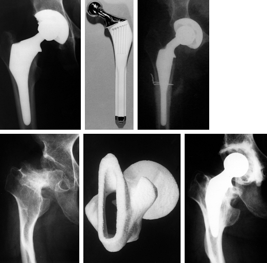
features (Fig. 100.28). Even if an
off-the-shelf hip is used for the more “normal” anatomies, custom stems
may still be used for abnormal situations. For revision hip
replacements, the variations in the proximal shape after removal of the
original stem, the diameter and curvature of the diaphysis below that
region, and the required location of the femoral head are so great that
a custom approach has a strong justification. Indications for custom
hip replacements are:
 |
|
Figure 100.28. Examples of custom hips used in primary cases, in which the anatomy ranged from normal to grossly abnormal. Top left: A custom hip used for normal anatomy. Top right:
Subtrochanteric osteotomy in a 90° anteversion congenital dislocated hip using longitudinal cutting flutes across the osteotomy. Bottom: Grossly abnormal geometry for which CT scans were used to design a tongue-shaped stem and a stereolithographic plastic model was made for preoperative trials. |
-
Congenital dislocated hip (CDH), in which
the femoral anteversion is in the range of approximately 30° to 60°.
The custom stem is designed to fit the canal closely and to restore the
normal 15° to 20° of anteversion. -
CDH in which the femoral anteversion is
in excess of approximately 60°. Here, a subtrochanteric osteotomy is
performed, the upper femur is rotated correctly at surgery, and the
custom stem is designed with longitudinal cutting flutes to provide
torsional stability across the osteotomy site (Fig. 100.28). -
CDH, juvenile rheumatoid arthritis (JRA),
or other conditions in which the hip is exceptionally small or has
severely abnormal anatomy (Fig. 100.28). -
In hips that are extremely large, or with
large canals, for which the custom hip is made hollow or slotted to
reduce the bending stiffness. -
After osteotomy, trauma, or other
conditions, with abnormal geometry, sometimes requiring an osteotomy at
surgery to restore normal geometrical relations -
Canals with extreme bowing in either the
AP or ML views or with an overhanging greater trochanter, requiring a
“banana-shaped” stem -
In revisions due to the wide range of
bony conditions, proximal shape and bone loss, stem length required,
anterior bow, distal diameter, and relation between the proximal and
distal dimensions. A graduated approach is especially appropriate for
revision hip replacements, as described earlier (Fig. 100.27).
A number of commercially available software packages can be used to
contour the inside and outside cortical bone boundaries, from which a
3-D model of the bone can be generated. The internal contouring
requires definition of a suitable Hounsfield number (a value signifying
bone density, where 100 equals water and 1000 equals cortical bone)
distinguishing the boundary between cancellous and cortical bone. For
purposes of reaming and rasping, a value of 500 to 600 has been shown
to be suitable. Another method for determining the shape of the femoral
canal that is more direct and less expensive but is restricted to
femurs of relatively normal shape is to use scaled AP and ML
radiographs (119). The canal outlines are
digitized and then a 3-D computer model of the “average femur” is
numerically distorted so that its canal outline fits that of the
specific femur. This method has been shown to be accurate to better
than 1 mm in the regions where a close stem fit is required.
is needed to design the stem to a particular scheme. For example, it
can be assumed that distal reaming and proximal rasping are performed
to produce a more geometric shape for ease of manufacture and surgery.
The general principle is such that the major load transmission occurs
proximally (110), which results in the following ideal features:
-
Medial, lateral, and anterior flares.
-
A collar with a coating for osseointegration.
-
A close-fitting proximal stem with an osseointegration coating.
-
Proximal macrogrooves to minimize
micromotion and provide additional bony stability should there be any
deterioration of an HA coating -
A relatively short and smooth distal stem to restrict its function to controlling bending rather than transmitting axial forces.
custom hip replacements, prewritten computer numerically controlled
(CNC) software is required. This software provides instructions to a
milling machine to produce the stem from a bar of preformed material.
The end result is an integrated software package that covers both the
design and manufacturing stages.
custom hip system compared with an off-the-shelf system is to assume
that accuracy of fit is the single criterion for comparison, and then
to determine how many off-the-shelf
sizes
would be needed to fit the general population of femurs to a given
accuracy. This requires that the most ideal set of sizes for the
off-the-shelf system be synthesized. The problem can be solved in the
following way:
-
Produce a “training set” of approximately
100 successive osteoarthritic cases for which custom hip replacements
have been produced, excluding shapes that clearly are outliers. -
Define the shape of the stem by p geometric variables, such as coordinates of numerous key points around the stem periphery.
-
Use “principal component analysis” to reduce the variables, using linear combinations of the variables that best express the p-dimensional scatterplot of the original variables
-
Synthesize an n-sized system such that if n = 1, that is the geometric mean, and if n > 1, the sizes synthesized provide the best fit for the largest number of the training set.
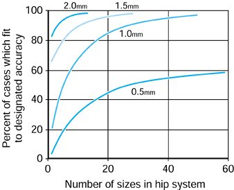
can be produced. If an accuracy of fit of 0.5 mm or better between the
stem and the bone were required, then a 40-sized system would achieve
this in just under 50% of all cases. However, if a 1 mm accuracy were
satisfactory, a 20-sized system would deal with more than 80% of all
cases. Virtually all cases could be dealt with using a 10-sized system
if only 1.5 or 2 mm accuracy were required.
 |
|
Figure 100.29.
Principal component analysis was used to synthesize best fit off-the-shelf hip systems with different numbers of sizes in the system. The percent of cases in the general population fitted to the specified accuracy is shown. |
replacement, namely surface replacement, the problem of fit is greatly
simplified. Such an approach can be classified as a conservative hip,
which can include several forms. A conservative hip is one that
involves fixation to the femur and acetabulum such that its removal for
any reason would allow the placement of standard primary hip components
with little compromise. Early examples of conservative hips are the
Aufranc cup arthroplasty and the various femoral head replacements with
short pegs, such as the Judet (212). From the
1970s to the present, various surface replacements have been attempted
using combinations of metal, ceramic and polyethylene for the
components, and press-fit, cement, porous, and HA for fixation. There
have been several problems with surface replacement to date:
-
The bone has remodeled inside the head to exaggerate the load transmission to the medial calcar, as predicted by FEA (Fig. 100.30).
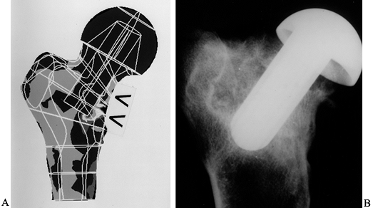 Figure 100.30. A:
The FEA analysis (Von Mises stress) shows decreased bone stress under
the head and increased stress in the medial calcar region. B:
The radiograph shows a conservative hip after 1 year in a goat, showing
bone resorption under the head, and new trabeculae where the stem is
close to the lateral cortex. -
Subsequent degradation of the implant–bone interface and overall loosening.
-
Fracture of the neck level with the rim
of the head component. The risk can be minimized by avoiding excess
reaming, as well as by details of component design. -
Excessive reaming of the socket to
accommodate sufficient thickness of UHMWPE. This has been solved by
using thin shells of a cobalt-chrome (Co-Cr) alloy, a metal-on-metal
bearing -
In cases of avascular necrosis of the femoral head.
A modification to a standard surface replacement is Townley’s TARA
design. This design removes most of the head, greatly reducing the
trabecular remodeling problem, whereas the short stem improves
stability. Thrust-plate designs (e.g., Wiles, Huggler and Jacob) have
met with some success in clinical follow-up, and further improvements
to this type are possible by using surface textures and coatings for
osseointegration. Advantages of this configuration are that good
initial stability can be obtained to allow for osseointegration, and a
normal modular head can be used. A key issue is that a proportion of
the varus bending is transmitted by the neck collar and by the lateral
plate because this has important remodeling consequences. Variants of
the thrust-plate design use different fixation at the neck resection
level, within the neck itself, and at the lateral cortex. FEA of hip
stems with a lateral flare indicates that, for a high neck cut, the
stem carries only a small bending moment, allowing its length to be
shortened considerably. This provides the possibility of a “proximal
plug” type of conservative hip. In this type, osseointegration can
occur over a large surface area. Preserving part of the femoral neck
for bone support is used in the Mayo conservative hip design (Zimmer,
Inc., Warsaw, IN) and in the Pipino hip. Other conservative hip schemes
include metal shrouds that cover regions of the outer proximal femur.
Such designs could have application for abnormal femoral geometries and
even for some revisions. From the acetabular perspective, those
conservative designs that incorporate a femoral
trunnion to use a standard modular head have an advantage for restoring the required head offset.
 |
|
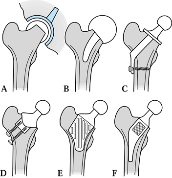
Figure 100.31. Different designs of conservative hip: (A) metal-on-metal surface replacement (Amstutz, McMinn); (B) capping design with stem (Townley TARA); (C) thrust plate (Huggler-Jacob, Wiles); (D) stemless design (Munting & Verhelpen); (E) proximal CAD-CAM (Santori-Walker); (F) Mayo Conservative Hip (Morrey).
|
stems with each other can be divided into laboratory studies and
clinical evaluations.
view, sagittal view, and the sectional fits, from a given stem size
range, in a representative selection of femurs. The goal with cemented
stems is to achieve a uniform cement mantle thickness around each cross
section, as well as minimum values of around 2 to 3 mm from distal to
proximal. For uncemented stems, the goal is to achieve stem–cortical
contact at those areas determined by the design philosophy, such as
around the entire distal stem or on the lateral and medial flares. From
a practical point of view, contact can be considered to be within a
defined tolerance level such as 0.5 or 1.0 mm (119).
In actual evaluations of this type on typical uncemented stems, it has
been found that there is only a small percentage of contact with
cortical bone.
component is fitted into a plastic or cadaveric bone, cyclic forces are
applied to
the femoral head in a test machine, and the stem–bone motion is measured over time (193).
It has been found that the stem subsides progressively, usually
reaching an asymptotic limit after a few hundred cycles. The total
subsidence is called “migration.” Thereafter, there is a cyclic elastic
deformation between the stem and the bone, termed “micromotion.” The
values of micromotion are usually in the range of 10-200 µm (109).
It is estimated that a value of about 50 µm is acceptable before
interface bone resorption would occur. Generally, better fit, a more
anatomic stem, the presence of a lateral flare, and more cortical
contact produce less migration and micromotion. To compare different
stem designs, use of the same artificial femurs (although it provides
reproducibility) might prejudice the results by being a better fit for
one particular design; hence, a range of femoral shapes is preferable.
The use of cadaveric bones is ideal for realistic geometry and bone
properties, but large numbers are needed for statistical significance
unless a small number of stems can be successively implanted into the
same femur without prejudice.
strains in the entire system can be determined. The data can then be
used to predict bone remodeling (201,230), interface failure, cement cracking, stem fracture, cement-stem debonding (210), and other factors (113).
A relatively recent advance is iterative analysis, in which the
material properties or a stem shape are changed as a result of the
first stress analysis (114). For example, the
elastic modulus values for the bone are changed to reflect the local
stresses where a region of stem causing a stress concentration is
smoothed away. The FEA is then rerun, and the process is repeated until
a steady state is reached. Using this technique, the bone remodeling
over time can be simulated, predicting the amount of bone loss in the
steady-state situation. An initial proposal for a stem shape can be
successively modified to minimize an objective function of the stresses
at the interface and in the bone itself. The consequences of
progressive cement debonding can be studied. However, there is still
considerable skepticism concerning the ability of FEA to predict actual
in vivo behavior. Indeed, many models are
idealized, showing, for example complete stem–bone contact when, in
reality, there is a variable mixture of gaps, as well as cortical and
cancellous bone contact. Nevertheless, provided the model is
appropriate to the intended question, the FEA method is invaluable for
comparing different stems, using such criteria as the stresses,
strains, or strain energy density in the system (185).
The method involves placing small tantalum beads in the bone at the
time of surgery, identifying landmarks in the component, and taking
biplanar radiographs through a calibration cage (127,168).
Digitization of the points to obtain coordinates allows the 3-D
position of the component relative to the bone to be calculated to a
high degree of accuracy, approximately 0.3 mm and 0.3°. As well as
being used for migration over periods of several years, the “inducible”
displacement at a particular time has been measured when the patient
relaxes and then loads the leg. These data give an idea of the rigidity
of the implant–bone interface.
retrospective data, where radiographic and clinical data are available
for a long follow-up time (e.g., 10 years), simpler methods have been
developed using landmarks on the bone and component. In some methods,
accuracy is enhanced using mathematical corrections for different x-ray
orientations, as well as by using boundary detection methods.
Accuracies of 0.5 mm and 0.5° can be achieved. A typical example of
migration curves using such a method is shown in Figure 100.32.
It is important to specify when the initial (time zero) measurement was
taken because even the first few steps of weight bearing can cause as
much migration as in the subsequent 6 months.
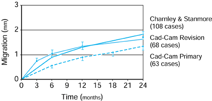 |
|
Figure 100.32. Migration versus time curves for three groups of hip stems. The CAD-CAM hips, such as those shown in Figure 100.27 and Figure 100.28, are compared with standard cemented hips. The migration curves are useful early indicators of longer term loosening rates.
|
uncemented hips, it has been found that the migration behavior in the
first 2 years correlates with loosening and radiolucency
in the longer term (133,222).
In particular, stems that are “continuous migrators,” that is, those
for which the migration rate at 2 years has not reduced to a very small
level, usually go on to “clinical loosening” during the following few
years. Hence, the method is invaluable for evaluating new hip designs
in a short time period. However, it must be recognized that longer term
effects such as socket wear, wear of the stem surface, fracture of the
cement mantle and of the stem itself, and corrosion or fretting at
interfaces are not addressed in such a short study.
the total bone mineral surrounding the implant, the proximomedial
region being of particular interest. The method is quantitative, unlike
radiographic data from which only general impressions of bone density,
or relative density, can be obtained (201).
Great care is needed in the interpretation of DEXA data. Bone density
can decrease in the postoperative months owing to the patient’s a low
activity level, and drugs can also have an effect. Large bone density
changes are often apparent only after several years, although 2-year
data would identify an implant with severe changes. Another factor is
that whereas subsequent changes in bone density can depend on the
initial stresses, calculated, for example, by FEA, if radiolucency
subsequently develops due to interface problems, the stress
distribution on and in the bone can change as a result.
subsequent osteolysis and loosening are the major limitations to
durability of total hip replacements (69,98).
Literally millions of particles are released on every step. The
particles consist of granules released from the tops of asperities and
ridges, or fibrils pulled away as small filaments. Particle size ranges
from 0.1 to 1 µm (107). The wear rates,
measured as the linear penetration into the socket, have averaged 0.05
to 0.1 mm per year for 22 mm joints, but the ranges in given series
have varied considerably (96). Determining the
effect of different variables on wear rate is difficult. In the
laboratory, the test conditions are greatly simplified, but aging
effects of the materials that occur in the body are not easily
reproduced. In vivo, there are numerous variables, many of which cannot
be accurately quantified. The main factors that affect the wear factor
and the rate of wear in total hip replacements are the diameter (149), surface finish, and material of the femoral head, as well as polyethylene processing and patient factors.
-
The Diameter of the Femoral Head. From the basic wear equations,wear rate = wear factor × load × sliding velocitywear volume = wear factor × load × sliding distancethe volume of wear is proportional to the diameter, and
the penetration is inversely proportional to the diameter of the
femoral head. Penetration into the socket in itself is not a problem
except when it begins to cause impingement, which can then loosen the
socket or result in dislocation. For 22 mm heads, these problems may
occur in longer follow-ups in heavy and active patients if the wear
factor is unusually high. It is noted that the wear equations assume
that the wear rate is independent of both surface area and contact
pressure, which may be a reasonable assumption for the ranges
encountered in hip joints (148,149). -
Surface Finish of the Head. Metallic femoral heads are manufactured with an exceedingly high polish of Ra value 0.01 to 0.02 µm. Ra is the mean value of the peaks and troughs with respect to a mean line (82).
In a new head, asperities, projecting from the surface, are not
present, except those made of materials such as cast cobalt-chrome.
Hard carbides at grain boundaries can resist polishing and be slightly
prominent. However, at surgery, the head can become scratched owing to
the impingement of instruments or hard particles embedded in the
impactor. In the patient, the head can become scratched by hard
particles from a number of sources: The UHMWPE can have contaminants;
the cement can release barium sulfate; the stem surface can shed
metallic debris or HA from coatings (26); or
bone particles can be present from surgery. The head itself can release
hard particles due to rubbing. As well as becoming temporarily trapped
between the bearing surfaces, particles can embed in the plastic,
causing multiple scratches on the head. The end result is that the
number of scratches on the head can accumulate over time. Typically,
the Ra value of retrieved heads compared
with new heads is two to three times higher for cobalt-chrome, higher
still for stainless steel, and highest for titanium alloy. In contrast,
the Ra value of ceramic heads changes
little over time. Scratches with cutting edges above the mean are the
most damaging, however. Over time, the wear factor K
will increase due to the scratching. However, the penetration rate into
sockets over time may still approximate to linear if the the patient
gradually reduces his or her activity level. -
Femoral Head Material.
In general, the harder and more wettable the material, and the better
the initial surface finish, the less the wear. Alumina ceramics against
UHMWPE have had a long history of clinical use and have shown wear
rates approximately half those of metal on UHMWPE, which has been
confirmed in hip simulator studies (237).
Zirconia ceramics have a similar record, although with shorter
follow-up at this time. However, zirconia is tougher than alumina and
would probably be recommended over alumina. Alumina ceramic-on-ceramic
bearings have shown exceedingly low wear rates, one to two orders of
magnitude lower in volume
P.2598
than
for metal or ceramic on UHMWPE. Zirconia-on-zirconia is not viable. The
main drawbacks of ceramics are that stringent tolerances are required
for the trunnions and for the bearing geometry itself, and a number of
breakages of ceramic heads have been reported, although the incidence
is well below 1%. Overall, the use of ceramic bearings from proven
sources offer definite advantages, especially for younger and more
active patients. Metal-on-metal bearings, using cobalt-chrome alloys,
have likewise shown exceedingly low volumetric wear over long time
periods. The reservations against more widespread use of these alloys
are the unknown long-term systemic effects of metallic ions, although
no adverse effects have yet been demonstrated in McKee-Farrar hip
replacements, which have had more than 2 decades of follow-up.
Metal-on-metal components can be designed with thin sections, which is
an advantage for surface replacement hips. -
Processing of Polyethylene.
In recent years, a great deal has been learned about the effects of
gamma irradiation, most notably molecular chain scission and
cross-linking (81). The latter can be due to
oxidation over time when components are stored for several years before
use or in service conditions. This factor, in turn, causes an increase
in density, a degradation of mechanical properties, and a reduction in
wear resistance. In such cases, retrieved sockets have shown a “white
band” of degraded polyethylene at or just below the surface. In
laboratory tests, the wear factor increases progressively with
oxidation level. At this time, when gamma-irradiation is used for
sterilization, the irradiation, together with the packaging, is carried
out in an inert atmosphere to avoid the effect of oxygen. Other
sterilization methods, such as ethylene oxide (ETO) and gas plasma,
avoid chain scission and oxidation, and evidently reduce the wear
factor. However, more recently, methods for minimizing the progress of
oxidation have been developed. The free radicals produced by
gamma-irradiation or by electron beam irradiation have been
cross-linked by various postirradiation treatments such as controlled
heating. The reductions in the wear factor have been dramatic, as
measured in hip-simulating machines. However, with some processing
methods, there is a reduction in mechanical properties so that suitable
fatigue testing of components is needed. -
Patient Factors.
The wear rate will increase with the weight and activity level of the
patient, and even the type of activity might have an effect. However,
in radiographic studies of wear penetration, or studies of retrieved
sockets, obtaining significance for a particular variable has proven
difficult because of the effects of many other variables and the
unknowns involved. Care must be taken to distinguish between wear
factor K, which is a constant for that
bearing (as long as the bearing does not change); wear rate, which
depends on weight and activity level; and wear volume, which is the
average wear rate times time.
measure wear rates. Today, data from such machines are a requirement
for the introduction of a new bearing combination. The proposed test
method by the International Organization for Standardization (ISO)
includes
-
A physiologic single-axis force cycle in a direction fixed in the acetabulum.
-
Three independent motion curves applied to the femur: flexion-extension, inward-outward rotation, and abduction-adduction (Fig. 100.4 and Fig. 100.20).
-
Twenty-five percent calf serum at 37°C.
-
Tests run at 1 Hz for 5 million cycles
-
Dimensional and weight changes measured at intervals.
conditions and to allow for comparative data between different
laboratories. No single test can, for practical reasons, reproduce
physiologic conditions, which involve a range of activities and a host
of other variables. The wide range of conditions in the patient
population means that the results of a test must be viewed
statistically and not in an absolute sense. A comparative test of a new
bearing against a known standard is therefore necessary. Another factor
is that, as with all wear tests, there can be a wide spread of results
from nominally the same bearing, which has led to the requirement for
multichannel machines (Fig. 100.33).
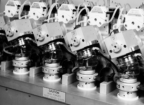 |
|
Figure 100.33.
A multistation AMTI-Boston hip simulating machine for long-term hip wear testing. The machine includes computer monitoring of the input forces and motions as well as other test parameters. (Photo courtesy Advanced Medical Technology, Inc., Watertown, MA.) |
-
The femur and acetabulum are either anatomically positioned (ideal for particle transport) or inverted (easier experimentally).
-
The force is applied relative to the socket or to the femur (in reality, the force is more closely aligned with the femur)
-
Independent motions about one, two, or
three axes are applied. To assess this motion, the paths of multiple
points on the femoral head traversing over the plastic socket can be
mapped (211). Only for three independent
motions do the patterns of the points resemble the physiologic
patterns, namely loops that cross over each other. This is embodied in
the present AMTI (Advanced Medical Technology, Inc., Watertown, MA)
machine. However, two motions, as long as they are not in phase, will
produce crossing loops but of different shape that can achieve similar
wear rates. This type of motion applies to the McKellop and to the
recent Leeds machines. Single-axis motion is inadequate in that
straight or curved
P.2599
tracks are produced that do not cross over one another, and hence the wear rates are too low.
to carrying out tests under ideal conditions, more adverse conditions
need to be addressed. The effect on the wear rate of scratches on the
femoral head or of hard particles introduced into the fluid are
particularly important.
derived from the measurements of “passive motion” of knee specimens
when the external forces are small (228). The
tibia has either been passively flexed and held at successive flexion
angles, or a small flexion moment has been applied, balanced by a force
in the quadriceps (97,183).
The motion itself has been described in several different ways, which
has led to a number of misunderstandings. The “contact points” are
defined as the common tangent of the femoral and tibial outlines, as
seen on radiographs (although in reality only the bone outlines and not
the cartilage outlines can be seen). These contact points displace
posteriorly, with the lateral contact point moving much more than the
medial (134,183) (Fig. 100.34).
If the actual contact areas were plotted, however, although the areas
would follow the same trend as the “points,” it would be difficult to
define a point directly from the areas because the areas are of
irregular shape and occur on both the cartilage and the menisci (2).
Motion can also be described by defining axes in the femur, the
transverse axis being through the centers of the lateral and medial
posterior femoral condyles, or the epicondylar line. If the motion of
the femoral origin at the center of the femur were plotted as a
function of flexion, it, too, would move posteriorly with flexion,
whereas the transverse x-axis would tilt slightly. This rigid body
motion would not be the same as that determined from the contact
points. For example, in a total knee replacement (TKR) seen in the
sagittal view, it can readily be observed that if the tibial surface is
dished, the contact point motion is much greater than the rigid body
motion.
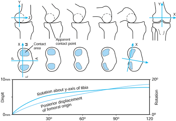 |
|
Figure 100.34. Three methods for describing passive knee motion. Top: The contact points defined by the common tangent. Center:
The contact areas. Lower: Rigid body motion of the femur relative to the tibia, based on axes defined in the femur and tibia. (Data from Rovick JS, Reuben JD, Schrager RJ, Walker PS. Relation Between Knee Motion and Ligament Length Patterns. Clin Biomech 1991;6:213.) |
As the knee is flexed from 0° to 120°, there is a posterior femoral
displacement and internal tibial rotation about its y-axis. There is
also a valgus rotation of the femur as the lateral femoral condyle
moves down the slope of the tibial plateau. This motion is governed by
the shape of the condylar surfaces, the different mobility of the
menisci on the lateral and medial sides (219), and the locations and stiffnesses of the cruciate and collateral (especially the medial) ligaments (5,41,88,89,183,199,207,241). This “passive motion” of the knee is useful for describing a middle path of knee motion for reference purposes.
-
An AP force or an internal-external torque is applied to the tibia about its y-axis at a given flexion angle (88,229) (Fig. 100.35). This produces displacements and rotations,
P.2600
which are termed laxity (108,123). The laxity is reasonably constant from about 30° to 120° of flexion but reduces as the knee is extended from 30°. An envelope of passive motion, defined as the boundaries within which the knee position can lie (24,25), is thus obtained.![]() Figure 100.35.
Figure 100.35.
The torque-rotation curves at different flexion angles describe the
rotational laxity of the knee. A composite of the rotations describes
the envelope of knee motion. Note that the x-axis represents the
neutral rotation at that angle of flexion. The neutral positions
relative to zero flexion change at subsequent flexion angles. -
An AP force is applied to the tibia along its z-axis, and then
an internal-external torque about the y-axis is applied. The rotational
laxity is reduced. Similarly, if the torque is applied first, the AP
laxity is reduced. This is termed coupled motion (143,172). In the extreme positions, the laxities can be reduced to very small values -
A compressive force is applied along the tibial y-axis. The laxities are now reduced, AP laxity (108) more so than rotational laxity (147).
The mechanism is that the dishing of the joint surfaces and the
deformation of the surfaces require that the joint displace upward to
move from its neutral position, thus requiring energy input. In the
normal knee, frictional effects due to the compressive force are small.
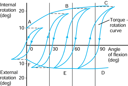
the knee motion occurs within the envelopes of laxity. An infinite
number of motion paths is possible; these paths are likely to vary even
between successive steps (164). The major factors that determine the actual motion path are the external forces and the muscle forces (138).
Whereas the principal force direction across the knee are along the
long axis of the tibia, the combination of the applied forces results
in shear forces and torques (Fig. 100.36).
These force components have been calculated using measured values of
the foot-to-ground force, the limb segment kinematics, and
electromyography (EMG) data of muscle action, input to
a knee model (136,155,156 and 157). In a recent study, telemetry data from an instrumented distal femoral replacement was used (206).
During walking, there are three peak forces of 2 to 3 BW. The shear
forces act in both anterior and posterior directions, with posterior
being predominant, in a direction so as to tense the PCL. The torque is
predominantly internal, the effect being to move the lateral tibial
plateau forward. The forces do not increase dramatically for ascending
and descending stairs, the largest increase of about 15% in the
compressive force occurring in descending stairs (156).
The patellofemoral forces are just less than half BW in walking but
reach approximately 1 BW or more in rising from a chair or climbing
stairs. The axial torques in level walking and on stairs are in the
range of 6 to 8 N·m.
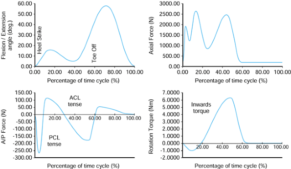 |
|
Figure 100.36.
The flexion angle, forces, and moments acting across the knee during normal walking, as specified in a current ISO-proposed standard for knee-simulating machines. These forces are distributed to the joint surfaces and to the ligaments. |
bearing surfaces using metal and plastic components, positioned so as
to restore the neutral alignment of the knee and achieve the correct
tensions in the ligaments (121). The simplest
form is a compartmental type (a “uni”), which is applicable if the
patellofemoral surfaces do not require replacement (55).
Most often, only the medial side is required, but replacement of both
sides as an alternative to a TKR has been used extensively in some
centers. Some of the issues concerning compartmental knees are the
following:
-
When both the anterior cruciate ligament
(ACL) and PCL are present and the components are correctly sized and
positioned, the function is close to normal (231). -
When the ACL is absent (19), abnormal motion and even instability occur (92).
-
Most designs have had a close-to-flat tibial surface, with a high sensitivity to the slope in the sagittal plane.
-
The flat tibial surface, thin plastic, and metal backing have led to severe wear problems in some designs.
-
Molded polyethylene flat components that
are not metal backed have survived for long periods (up to 20 years)
without serious wear (102). -
Loosening has been a problem, especially when the subchondral bone has been removed and there has been excessive AP sliding
-
Surgical placement has been difficult in the absence of a precise instrumentation system.
on the medial side is small, it appears logical to provide a dished
tibial surface, which would alleviate a number of the above problems.
Improved designs and instrumentation, coupled with small incisions,
present an important opportunity for outpatient surgery in the
appropriate indications.
compartments are able to provide stable fixation, are self-aligning,
and incorporate the patellofemoral surfaces; for these reasons, such
designs are the most frequently
used.
A fundamental principle of condylar replacement is that the artificial
surfaces are designed such that, in combination with the remaining
joint structures, the laxity and stability characteristics are similar
to those of the normal intact knee (144). In general terms, if all of the ligaments are preserved, the tibial surface requires only shallow dishing (Fig. 100.37).
If the ACL is absent, posterior curvature is required (although in most
designs there is insufficient curvature to compensate for the ACL). If
both cruciate ligaments are absent, posterior and anterior curvatures
are required (85).
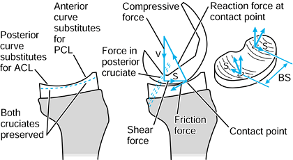 |
|
Figure 100.37. The principles of the total condylar type of TKR. Left: Geometry of the tibial surface, depending on whether the cruciate ligaments are present or absent. Center: When there is a compressive force and a shear force on the femur, these forces are carried by the surfaces and the ligaments.Right: Torque Q is carried by the shear force components S acting at distance BS, Q = S × BS.
|
ligaments and, to a lesser extent, other ligaments and soft tissues,
and the reaction forces at the joint surfaces (19). The ACL is more tense in early flexion, and the PCL is more tense in high flexion (183).
The fraction of the shear force carried by the cruciate ligaments
depends on the tibial surface geometry, the location of the “bottom of
the dish,” and the placement of the components. Even modest dishing of
the tibial surface (e.g., sagittal radius, 70 to 80 mm) provides
considerable stability, especially when high compressive forces of 2 to
3 BW are exerted (144,214).
In TKRs in which the PCL is preserved, the fraction of the shear force
carried by the PCL depends on the curvature of the tibial surface, the
curvature of the interfacing femoral surface (which depends on the
angle of flexion), the location of the bottom of the tibial dish, the
tightness of the PCL (which depends on the surgery), and the angle of
flexion (89). In practice, the PCL, especially
the anterior fibers, carry an increasing proportion of the anterior
shear force with flexion (129). The different schemes for condylar TKR design have advantages and disadvantages:
-
Combined ACL and PCL preservation
(assuming the knee has both) requires condylar shapes and surgical
placement within approximately 2 mm of ideal to be effective. The
tibial component must leave space for both ligaments, and surgical
exposure is more restricted. -
PCL preservation alone may result in an abnormally posterior contact point in early flexion (68), and there is no mechanism for producing anterior displacement of the femur as the knee extends.
-
ACL and PCL sacrifice requires condylar
shapes (or cams) with excessive rotational constraint under
weight-bearing conditions. The AP displacement is limited, although an
intercondylar cam may produce posterior femoral motion in high flexion -
A valid and reproducible method is needed
for the bone cuts and for performing ligament releases to achieve ideal
kinematic and stability characteristics. This condition applies more
especially when one or both cruciate ligaments are preserved.
dished condylar surfaces, embodied in the original Total Condylar
(Howmedica, Rutherford, NJ) (213,215,228) and in a number of other later designs, is shown in Figure 100.37. If there is a compressive force V acting down the long axis of the tibia, the femoral component locates at the bottom of the tibial dish. If a shear force S is superimposed, the femoral component displaces anteriorly such that the reaction force at the contact point exactly balances V and S.
The contact point displacement is greater than the rigid body
displacement. A torque applied to the tibia is equilibrated by an
anterior displacement of one side of the knee and a posterior
displacement of the other. The torque Q carried by the surfaces is S × BS, where BS
is the bearing spacing. The total condylar type of design thus provides
both stability and laxity, and has the advantages of moderate
conformity for low wear, simplicity, and ease of surgery.
concept is an evolution of the Freeman and Freeman-Samuelson (Protek)
designs (86). The medial side is almost fully
conforming, whereas the lateral side has low conformity. This has the
potential advantages of achieving physiologic motion and reducing wear
on the more heavily loaded medial side.
In neutral rotation, an AP laxity test, in which an anterior shear
force is applied to the femur followed by a posterior shear force,
produces anterior and posterior femoral displacements. As shown in Figure 100.38,
when there is greater conformity anteriorly, the anterior femoral
displacement is less. When rotation is superimposed, one femoral
condyle moves up the posterior curve. Because of the greater anterior
conformity, the movement up this curve is less than that at the
posterior
and, hence, there is a posterior shift in the neutral femoral position.
When the AP laxity test is now carried out, the AP displacement is
reduced. The more rotation that is superimposed, the less is the AP
laxity and the more is the shift in the neutral position. If the femur
is now flexed, the smaller posterior femoral radius is now in contact
with the tibia, and the laxity is reduced. However, as shown in the
geometric drawings of the sagittal femoral outline, the neutral
position of the femur is now shifted anteriorly.
These shifts in the neutral position, which are primarily dependent on
femoral geometry, have an important effect on soft-tissue tensions and
kinematics.
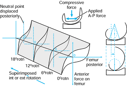 |
|
Figure 100.38.
Coupled motions, showing the effect of superimposed internal-external rotation on AP laxity. As rotation is increased, the AP laxity decreases and the neutral point of the femur moves posteriorly. The geometric profile drawings show that in flexion the rigid body motion of the femur moves anteriorly due to the sagittal curvature, and the AP laxity is increased. |
The coefficient of friction for metal on polyethylene surfaces is 0.05
to 0.1. For a condylar prosthesis implanted in a knee, without
friction, the laxity curve would be strain stiffening (Fig. 100.14)
with a hysteresis loop. However, owing to friction when a compressive
force is acting and the shear force direction is reversed, as occurs
during the gait cycle, there is a “stick” period without motion. In
function, this will result in some erratic behavior of the motion, with
combinations of rolling, sliding, and stick.
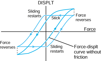 |
|
Figure 100.39. Friction has an important effect on motion, by reducing the total laxity and by causing “stick” periods.
|
that the geometric parameters of a TKR play an important role in
determining function and durability. The geometric considerations can
be broadly categorized as being in the sagittal plane or the frontal
plane.
-
The profile of the patellar flange replicates normal to produce correct quadriceps lever arms (7). Gait abnormalities (19) have been associated with profiles that are too prominent distal-anteriorly (8).
-
The distal radius of the femoral
component is larger than the posterior radius to provide greater
stability and larger contact areas in early flexion. -
If the posterior-distal transition angle
(PDTA) is about 20°, the large distal radius contacts the tibia during
the stance phase of gait, maintaining relatively low contact pressures.
However, this will result in a tendency for anterior sliding of the
femur after 20° (Fig. 100.38). -
The posterior radius is similar to the
anatomic radius (approximately 20 mm average) to maintain correct soft
tissue lengths. This will result in increased laxity in flexion
compared with extension, as in the normal knee. -
When the femur locates at the bottom of
the tibial dish the radius in early flexion, the femur and tibia are in
the correct anatomic relation to ensure normal patella and soft-tissue
mechanics -
As the knee moves to zero flexion and
into slight hyperextension, the contact point rolls anteriorly to
provide an increased lever arm for the hamstrings and gastrocnemius.
-
The bearing spacing (Fig. 100.40)
determines the varus-valgus moment before lift-off, and affects the
feasibility of interchangeability between different sizes in TKR
systems. A larger BS value is preferable.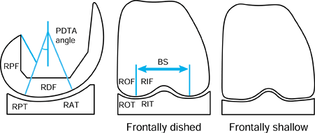 Figure 100.40.
Description of a condylar TKR using geometric parameters. These have an
important effect on function and durability. BS, bearing spacing
between the lowest points on the femoral condyles; PDTA, the angle of
transition between the distal and posterior radii; RAT, anterior tibial
radius; RDF, distal femoral radius; RIF, inner femoral radius; RIT,
inner tibial radius; ROF, outer femoral radius; ROT, outer tibial
radius; RPT, posterior tibial radius; RPF, posterior femoral radius. -
The inner femoral radius (RIF; Fig. 100.40) is determined by the requirement to provide an anatomical patellar groove.
-
The outer femoral radius (ROF; Fig. 100.40)
needs to be between approximately 25 mm and the sagittal tibial radius,
which is 55 to 80 mm in contemporary designs. This is required to avoid
the outside of the femoral condyles digging in during internal-external
rotation. -
A femorotibial radial clearance of only 1
to 2 mm produces elliptically shaped contact areas with relatively low
contact stresses. -
For a given clearance between the femoral and tibial radii, larger outer radii (ROF, ROT; Fig. 100.40) have the advantage of a larger area of contact and reduced contact stresses.
-
When lateral lift-off occurs, the contact
point for large radius surfaces will roll medially, counteracting
further lift-off. In extreme cases, there may be some tendency to ML
slipping. For a given clearance, there is a critical varus angle at
which digging in occurs. -
When lateral lift-off occurs, the small
radius surfaces rotates about the center of curvature and the contact
point remains constant. ML stability is maintained -
For a given clearance between the femoral and tibial radii, surfaces of larger radius provide increased rotational laxity.
However, other designs have shown serious problems, such as instability
(including ML), tibial baseplate fracture, excessive wear and
deformation, patella subluxation, limited flexion, and component
loosening. In many cases, the problems have been related to
unsatisfactory geometric features of design; in other cases, alignment
has been the main problem (169,208).
is provided by the articular surfaces and the retained ligaments. The
motion of the femorotibial contact point is hence determined by these
factors, in response to the external forces and the muscle forces. As
indicated previously, designs with shallow tibial surfaces and
preservation of both cruciate ligaments have the theoretical capability
of reproducing normal kinematics. Fluoroscopic techniques have been
used to record relative tibial and femoral knee motion during a range
of activities. The method involves sequential high-resolution
fluoroscopic images obtained in the sagittal plane. If the 3-D geometry
of the femoral and tibial components is known and input to the
computer, then the computer image can be moved into a 3-D orientation
so as to match the radiographic image. In this way, the relative 3-D
position of the femur on the tibia can be determined throughout the
activity. The accuracy of such methods is now better than 1 mm and 1°.
Interestingly, this method was originally developed for the military to
identify high-flying aircraft.
-
The smooth AP and rotation patterns
measured in passive knee motion are not reproduced during
weight-bearing activities, such as deep-knee bends and step climbing. -
The AP motion between the femur and the tibia is strongly influenced by the ground-to-foot and muscle forces.
-
There are considerable differences in the
AP motion between different individuals. Even the same individual
produces variable AP motion for the same activity at different times. -
TKRs with high femorotibial conformity in the sagittal plane show more reproducible AP motion
-
Condylar lift-off, mostly medial, occurs
often, and it is more frequent and of greater magnitude with
PCL-resecting devices and when the BS (Fig. 100.40) is low.
that control relative femorotibial motion in a more predictable way, at
least during part of the flexion range. One scheme for controlling the
kinematics is by the use of intercondylar cams.
is embodied in the Kinematic (now the Kinemax) Stabiliser (Howmedica,
Rutherford, NJ) (78) (Fig. 100.41),
which consists of cam surfaces that are in contact throughout flexion
and produce a progressively posterior movement of the femorotibial
contact point with increasing knee flexion. The second type is used in
the Posterior Stabilised Knee (Zimmer, Warsaw, IN), in which the cams
interact only after about 70° flexion (233), thereafter producing a large posterior displacement of the contact point. The aims of these particular designs were to:
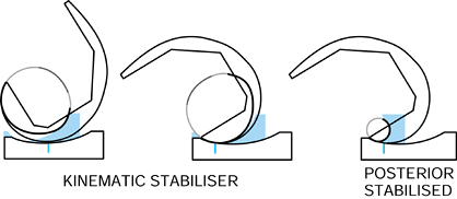 |
|
Figure 100.41. Examples of early guided-motion knees, in which certain phases of the AP motion are controlled by intercondylar cams. Top: Kinematic (now Kinemax) Stabiliser (Howmedica, Rutherford, NJ). Bottom: Posterior Stabilised Knee (Zimmer, Warsaw, IN).
|
-
Increase the quadriceps lever arm at high flexion angles.
-
Increase the range of flexion by preventing posterior impingement of bone and soft tissues
-
Prevent posterior tibial subluxation in flexion under the action of the hamstrings.
-
The height of the contact points on the
plastic cam should be minimized to minimize the rocking moments on the
tibial component, and to reduce the possibility of fracture of the
plastic post and component loosening. -
The cam should be shaped to allow internal-external rotation without digging in at the corners
-
The amount of elevation of the femoral component before dislocation occurs (“hop height”) should be maximized.
the condylar bearing surfaces themselves, are to provide ideal knee
kinematics, the following criteria can be added:
-
The device should control the location of
the femorotibial contact points in the AP direction and
internal-external rotation throughout the flexion range but allow some
laxity about these contact points. -
The device should guide the contact
points posteriorly with flexion (especially on the lateral side) and
anteriorly with extension. -
The device should produce internal tibial rotation progressively with flexion and external rotation with extension.
and soft-tissue tensions to restore optimal function as closely as
possible. By using special computer programs (225), the designs shown in Figure 100.41 and other types of intercondylar guide surfaces with different patterns of motion control can be synthesized (Fig. 100.42). Another example is the Superstabiliser-CCK type (137,191,213).
(Superstabilizer is a product of Howmedica, Rutherford, NJ; CCK is a
constrained condylar knee manufactured by Zimmer, Warsaw, IN.) This is
designed primarily to carry varus-valgus moments, and hence, the
computer program is used to maximize the area and strength of the
plastic tibial post. In addition, it can be seen that the interaction
between the femoral and tibial guide surfaces produces anterior femoral
displacement toward extension and posterior displacement toward full
flexion.
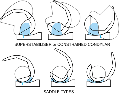 |
|
Figure 100.42. Intercondylar guide surfaces with different patterns of AP motion control. Top: Superstabiliser (Howmedica, Rutherford, NJ)—Constrained Condylar Knee (Zimmer, Warsaw, IN). Bottom: Saddle type with AP control in the second half of flexion (left), the mid-range of flexion (center) or in the first half of flexion (right).
|
guide surface is an eccentric circle and the tibial guide surface is a
saddle (225). This can provide AP motion control in different parts of the flexion range (Fig. 100.42).
By defining and varying geometric parameters of the above-mentioned
types, different AP control patterns can be achieved. In another design
using intercondylar guide surfaces (66), the
saddle moved the contact from anterior to posterior during flexion, the
second part of flexion using a ball-in-socket. In another design (76), the saddle shape was such as to induce pure rolling during flexion and extension.
femorotibial contact in early flexion and posterior contact in late
flexion have been achieved using separate pairs of bearing surfaces.
The TRAC (Biomet, Inc., Warsaw, IN) uses intercondylar guide surfaces,
shown at the lower left of Figure 100.42, to transfer the contact from the first pair of bearing surfaces to the second. The Bi-Articular
(Kyocera, Kyoto, Japan) uses conventional total condylar bearing
surfaces until about 90° of flexion. On further flexion, intercondylar
surfaces of spherical shape, which are posteriorly located, interact.
The goals are maximum flexion and freedom of internal-external rotation.
(usually medial). A “mobile bearing” is a plastic bearing that includes
both the medial and lateral compartments. A “mobile bearing knee” has
come to mean any unicompartmental or total knee replacement
incorporating a meniscal bearing or a mobile bearing (37). The purposes of a mobile bearing knee (Fig. 100.43) are to minimize the wear of the plastic and to allow relatively unrestrained motion to occur between the femur and the tibia.
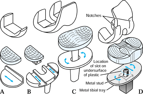 |
|
Figure 100.43. Schemes for mobile bearing knees: A: unicompartmental (Oxford Knee, Biomet, Inc., Warsaw, IN); B: LCS (Depuy-J&J, Warsaw, IN), or Minns (Zimmer, Warsaw, IN) with separate plastic components in tracks; C: LCS rotating platform; D: MBK (Zimmer, Warsaw, IN) with fully conforming femorotibial surfaces.
|
natural knee such that nonconforming main bearing surfaces, which allow
freedom of motion, have menisci interposed to increase the contact area
(2,219). The
deformability of the menisci allows for changing femorotibial geometry
during flexion while still maintaining a large contact area. The
constraint of a mobile bearing knee compared with a natural knee is
less on the medial side and more on the lateral side.
-
Complete conformity throughout the full
range of flexion. This is achieved in the Oxford (Biomet, Warsaw, IN)
unicompartmental design, using spherical surfaces (53).
However, this modular design does not provide for the patellofemoral
joint. The Polyzoides Rotaglide (Corin Orthopaedic, Gloucestershire,
United Kingdom) (173) has total condylar type
components, but the femoral and tibial bearing surfaces are spherical,
giving full contact throughout flexion from just anterior of the bottom
of the tibial dish to the posterior tibial surface. There is a normal
patellar flange. A recent design that achieves full contact from the
anterior to the posterior of the tibial bearing surface is the MBK
(Zimmer, Warsaw, IN) (225). This is achieved by notches in the medial and lateral sides of the femoral component (Fig. 100.43). The advantage of this scheme is the larger contact area and the resistance to anterior subluxation of the femur on the tibia. -
Complete conformity in early flexion but
partial conformity at higher flexion. One example is the LCS
(Depuy-J&J, Warsaw, IN) (37). The reason
for this compromise is to allow for a femoral component design of
reasonably anatomic sagittal geometry with a radius that is larger
distally than posteriorly. Full conformity is achieved during the major
part of a level walking cycle, whereas partial conformity is restricted
to the less frequent activities requiring higher flexion.
testing, it is not possible to assert which scheme will produce the
least wear and plastic damage over the long term. However, surface
wear, pitting, and delamination wear must all be considered in any
comparison.
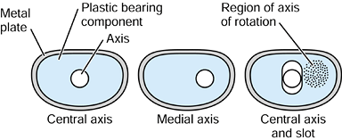 |
|
Figure 100.44.
For one-piece plastic components, there are several mechanical schemes for obtaining different femoral-tibial motions. For the axis plus slot, if the medial structures are tighter than the lateral, the axis of rotation can be variable and lie in the region found for the natural knee (shaded). |
-
The plastic menisci are separate and are
free to slide and rotate on their own metal plates (e.g., the Oxford).
Even though this allows for the maximum freedom of motion, there is the
possibility of bearing dislocation or excessive posterior overhang. In
this simple type of design, components with a minimum thickness of 4 mm
can be used. -
The plastic menisci are separate and
slide in curved (LCS) (DePuy-J&J, Warsaw, IN) or straight (Minns,
Zimmer, Swindon, UK) tracks in a one-piece metal baseplate. Suitable
clearances in the slots allow for combined sliding and rotation. The
possibility of bearing dislocation is reduced, but overhang is still
possible. Because of the slots, the overall component thickness has to
be increased. -
A one-piece mobile bearing is free to
rotate about a central pivot. This factor eliminates the uncertainty of
rotational placement at surgery and allows rotational freedom in
function. However, when rotation occurs, the lateral side moves
posteriorly and the medial side moves anteriorly, which does not
resemble anatomic motion where the contact on the medial side remains
reasonably constant. This problem can be solved by using a medial pivot
at the expense of requiring left and right components. -
A one-piece mobile bearing is free to
rotate and free to translate AP. This bearing can accommodate anatomic
motion, with an effective center of rotation on the medial side. The
posterior displacement during flexion can be provided by a retained PCL
or by muscle action. However, as with a fixed-bearing knee with a
shallow tibial surface, in early flexion, the femoral component may not
be sufficiently anterior.
are possible to achieve roll-back with flexion and even roll-forward
with extension. A posterior stabilized arrangement can be used, but
this would require partially conforming femorotibial bearing surfaces.
Guide surfaces, such as those described earlier, can interact between
the femoral component and the metal tibial baseplate. This is
applicable to either partially or fully conforming bearing geometry.
-
The kinematic analog of a meniscal
bearing knee (such as the Oxford used on the medial and lateral sides)
is a fixed bearing with shallow or flat tibial surfaces. In this case,
the mobile bearing is preferable because the fixed-bearing plastic is
liable to excessive deformation and wear in the long term owing to high
contact stresses. At the same time, if UHMWPE can be made with enhanced
resistance to wear and delamination, the two schemes become comparable -
The wear in a moderate-high conforming
fixed bearing may be comparable with that in a mobile bearing. The
fixed bearing, however, is too constrained in AP and rotation, whereas
the mobile bearing has increased laxity and a variable neutral
position, both of which are advantages.
no reliable data on the wear rates, and the types of particles
generated as a function of contact area and contact pressure. Hence,
comparisons between different designs must be determined by simulator
tests rather than automatically assuming that larger contact areas are
an advantage, as has been commonly done in the last decade.
been introduced, which reflects more the opportunity for inventive
design rather than extensive need. The largest numbers continue to be
used in Europe, whereas in the United States, the tendency is to use
the most conservative design whenever possible, even if substantial
soft-tissue balancing is required. The characteristics of a linked
design are:
-
Stability is provided in all degrees of
freedom, varus-valgus and hyperextension being particularly important,
although there can be some laxity (e.g., rotational) in one or more
degrees of freedom. -
A linkage of some type, such as a hinge, provides the stability and prevents subluxation or dissociation
-
Intramedullary stems are required for fixation.
the St. Georg Endo (Waldemar-Link, Germany) model, the Sheehan
(Howmedica, Rutherford, NJ), the Rotaflex (JJ Orthopaedics, Warsaw,
IN), and the PFC S-ROM
(J&J
Orthopaedics, Warsaw, IN). The bearing surfaces can be extended to the
full width of the knee, an advantage for reducing varus-valgus bending
moments on the linkage. The patellofemoral resurfacing has been absent
in some designs but ideally should be included. Advantages of the
intercondylar design are:
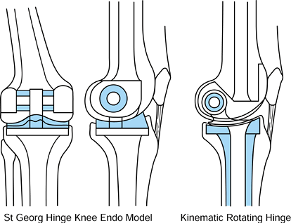 |
|
Figure 100.45. Different configurations of hinged designs. Left: the St. Georg (Waldemar-Link, Germany) fixed or rotating intercondylar hinge. Right: the Kinematic Rotating Hinge (Howmedica, Inc, Rutherford, NJ). Shaded areas indicate plastic.
|
-
Preservation of bone
-
The anatomic location of the axis of rotation.
-
The relatively restricted size of the bearing components, with an increased potential for wear and deformation.
-
The possibility of condylar fracture on each side
-
The difficulty of linking the components
at surgery, and the possibility of dislocation in extreme loading
conditions (in some designs).
bone resection, is the fixed hinge or rotating hinge. Placement is
achieved by resection of about 25 mm from the distal femoral condyles
and 10 mm from the upper tibia. An axle is then used to connect the
femoral and tibial components, usually with plastic bushings to act as
the bearing. The total thickness is determined by the required
dimensions of the axle and bushings, and the ideal placement of the
axle, which is close to the epicondylar line. A lower, or more
posterior, axle location will reduce bone resection but result in
abnormal tracking of the patella. It should be noted that the most
important requirement in the placement of hinged replacements is that
the patella locates at the correct level on the femoral flange with the
knee in extension.
for patients of low demand who would not overstress the fixation and
for whom flexion-extension motion is sufficient. Examples are the
Guépar (Benoist-Gerard), the St. Georg (Link), the Blauth (Allopro),
and the original Stanmore. The rotating hinge, however, results in a
more “natural” feel to the patient and can be more durable in the long
term. Examples are the Kinematic and Kinemax Rotating Hinges
(Osteonics-Howmedica, Rutherford, N.J.), the Finn (Biomet, Warsaw, IN),
the Noiles (J&J Orthopaedics, Warsaw, IN), and the SMILES (Stanmore
Implants Worldwide). More bone resection, however, is required to
accommodate the extra bearing surface. The rotation can be achieved by
a flat polished metal surface pivoted on a flat plastic surface, or by
a convex metal surface in a dished plastic surface. The convex metal
surface in a dished plastic surface is preferable because it provides a
“soft” limit to rotation, reducing the possibility of instability or
patellofemoral subluxation. Some medium- to long-term follow-up studies
of linked designs have shown durability comparable to that associated
with condylar replacements (32). That fact,
coupled with the relative ease of surgery and the immediate stability,
makes linked designs an attractive option for selected patients.
-
The plastic is thin at the sides, resulting in overall deformation of the component, especially in activities with high flexion.
-
If the femoral flange has an anatomic
profile (to accept a retained patella), the dome has two local areas of
high stress, which are subject to wear and deformation -
If the profile of the patellar flange is a circular arc to match the dome, a retained anatomic patella is a poor fit.
increased plastic thickness at the sides and larger contact areas in
the form of two “lines” rather than “points.” Finally, the gaussian
shape further increases both the thickness and the contact area. In all
of the designs, a medial offset to the peak is an advantage and
eliminates the need to use a smaller size of symmetric design and
medialize it. A rotating platform design produces the largest area of
contact and potentially the least wear and deformation, at the expense
of some extra thickness due to the metal backing and a second bearing
surface. An additional factor in area of contact is the shape of the
intercondylar cutout on the femoral component, as shown in Figure 100.46.
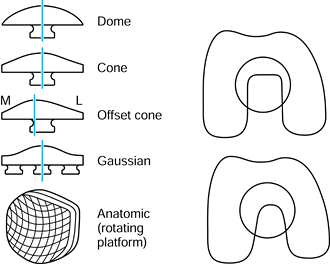 |
|
Figure 100.46.
Shapes of patellar component used in TKR (an “inset” patella is not shown). The narrower and more posterior the intercondylar cutout on the femoral component, the larger the contact area on the patella in high flexion. |
is more forgiving in alignment and that the other types are susceptible
to tilting and loading on the corners. In the front view, it can be
seen that, owing to the angle between the lines of action of the
patellar ligament and the quadriceps (the Q-angle), there will be
resultant tensile and lateral shear forces on the patella itself (Fig. 100.47). The actual direction of the forces depends on the relative forces in the different parts of the quadriceps (3,4,103,117).
In addition, there will be a compressive force between the patella
(whether the natural patella or a plastic replacement) and the patellar
flange, which increases with the flexion angle up to about 100° flexion
(4). A 3-D force analysis can be carried out, based on the sectional view shown in Figure 100.47. If the resultant compressive force is central, equal resultants act on the lateral and medial facets (Fig. 100.48).
However, in general, the lateral reaction force will be larger than the
medial owing to the laterally directed component of the quadriceps and
patellar tendon forces. As the Q-angle increases, the lateral force
will increase and the medial force will decrease. However, as long as
both forces are positive, the patella will be stable. At the point
where the medial force reaches zero, the patella will become unstable
and will be subject to tilting and subluxation. This is calculated to
occur at a Q-angle of approximately 12° (117).
Except in cases of extreme valgus, this is unlikely, and hence the cone
and gaussian patellar components are likely to be stable.
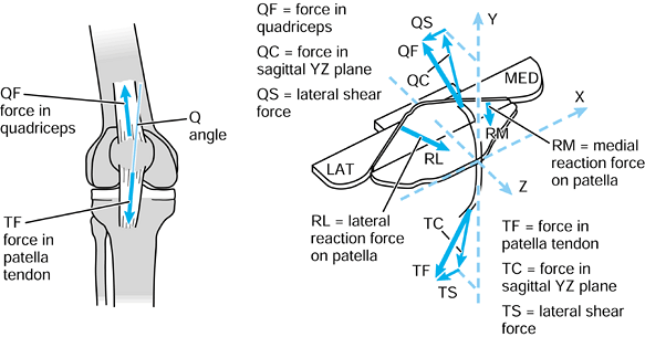 |
|
Figure 100.47.
The Q-angle between the quadriceps and patellar tendon forces results in a lateral shear force on the patella. The sectional view treats the patella as a free body (Fig. 100.9), from which the forces, including the lateral and medial facet forces, RL and RM, can be calculated. |
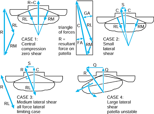 |
|
Figure 100.48.
The resultant forces between the patellar component and the femoral flange. As the lateral shear component is increased, a critical unstable situation is reached but at a high Q-angle. |
include cementation, press-fit fixation, porous-coating, and fixation
with various macroscopic surface finishes or mesh. Any of the
uncemented modes can include HA or other bioactive coating. The goals
are to minimize interface micromotion (17,220), avoid interface bone resorption, and maintain intimate bone contact (170).
An alternative goal, potentially achievable with press-fit fixation, is
to obtain a stable interface with a thin fibrous tissue layer or
velour-type material (154,224).
In cementing at surgery, if the cement is applied in a viscous state
with little pressure, the penetration will only be on the projecting
trabecular tips, allowing distraction to occur when local tensile
stresses are exerted (Fig. 100.49). In
contrast, penetration of 2 to 4 mm, such that transverse trabeculae are
engaged, results in small interface micromotion and an interface that
can remain stable for long time periods. The most uniform penetration
over the entire surface is achieved with cement applied by multiple
applications of a gun nozzle.
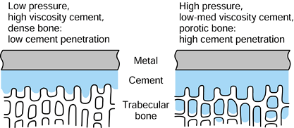 |
|
Figure 100.49. The interface conditions between cement and trabecular bone for low and high penetration of cement.
|
problem in metal-backed components but has occurred with all-plastic
components when there has been deformation due to poor or uneven bony
support or bone overload from malalignment (178).
Components with coatings, for which long-term fixation relies on
ingrowth or apposition of new bone, require initial fixation that is
sufficiently rigid for at least 2 to 3 months. Screws have been found
to be an advantage for tibial components, whereas for femoral
components (197), a tight AP fit has been
adequate. However, the use of screws carries the risk of screw-tray
fretting and of providing a track for wear debris particles, which
produce osteolytic cavities. Press-fit fixation requires suitable
macroscopic features and pegs to maintain a sufficiently low level of
interface micromotion (221). In many cases, a
stable fibrous tissue interface above a new subchondral layer has been
formed, but so far, press-fit fixation has shown a higher incidence of
loosening and pain than cementation.
These factors, in turn, directly affect the stress distribution over
the entire interface as well as the stresses in the bone itself (Fig. 100.50).
In the sagittal plane, if the contact is less than approximately 25%
from the edge, there will be excessive bone stresses beneath the load
and tensile stresses opposite to the load. The actual pressure
distribution at the interface reflects the foundation stiffness of the
trabecular bone, whereas the magnitude of the stresses depends on the
surface area of the component. The bone stiffness is modified in
arthritic conditions, usually by increased and decreased stiffness on
opposite compartments. CT studies show that, after realignment and
insertion of a TKR, whereas the strong bone reduces in strength toward
normal, the weak side gains in strength more slowly (118).
Except in conditions of extreme edge loading, metal-backed components
produce a more normal pressure distribution at the interface. In
all-plastic components, there is a high pressure region at the
interface beneath the contact area. Nevertheless, there is clinical
evidence that plastic components with sufficient thickness (e.g., 10
mm) and a strong central peg are viable in patients with low activity
levels and when there are no major bone defects or regions of
osteoporosis (178). Regarding overall pressure
distribution, central posts reduce the maximum interface stresses for
offset loading, such as varus (179), as well as being effective against shear forces (Fig. 100.51).
Design features located toward the periphery, such as pegs or keels,
especially when they are embedded in hard cancellous bone, are
effective against internal-external rotation (221).
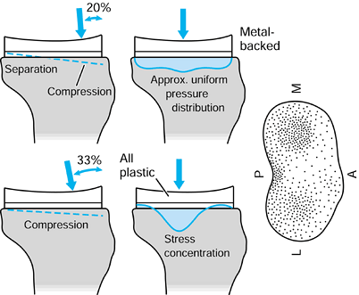 |
|
Figure 100.50.
Elastic deformations and interface stresses of tibial components on the upper tibia. The figure on the extreme right shows a typical foundation stiffness on the resected upper surface, which is usually modified in arthritic conditions. See text for details. |
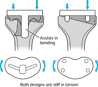 |
|
Figure 100.51. Design features to transmit varus moments and axial torques more effectively to the bone.
|
One millimeter tantalum beads are implanted in the component and in the
adjacent bone at surgery. Biplanar radiography at specific time
intervals, with mathematical analysis, produce the component–bone
movements or migrations over time. Continuous migrators after 1 to 2
years are predictive of future clinical loosening.
These augments can be screwed or cemented to the main components. For
larger defects, space fillers made from metal or plastic are an
alternative to bone grafting. Stems are useful for bypassing cavitary
defects, for protecting against fractures, for traversing fracture
sites or serious cortical defects, or for stabilizing allografts (179).
When the TKR design carries varus-valgus moments, intramedullary stems
are needed. In older patients, cemented stems are usually preferable,
but uncemented fluted stems should be used if there is sufficient
cortical thickness, in order to reduce the stress-shielding of the
cancellous bone near the joint (209).
Empirically, suitable stem lengths for Superstabiliser-CCK types of TKR
are 100 to 120 mm, and 120 to 150 mm for rotating and fixed hinges.
Revision of a failed cemented stem requires a new stem at least 50 mm
longer. In all cases, attention is needed to prevent the stem tip from
impacting the cortical wall, which frequently produces osteolysis,
penetration, and even bone fracture.
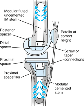 |
|
Figure 100.52.
Modular augments including spacers, space fillers, medial wedges (not shown), and stems; they are used in cases of bone loss including revisions. There is some stress protection of the distal femur and proximal tibia due to the stems. |
described earlier in the discussion of tribology. In this section, wear
mechanisms applied to TKR are discussed. These mechanisms have been
deduced from retrieval studies, principally from components that have
failed due to instability or loosening (18,27,28,29,60,61,63,139,234). Examples of wear in a range of retrieved TKR components are shown in Figure 100.53. Deformation frequently occurs in dome-shaped patellar components when they are used in anatomically shaped grooves (Fig. 100.54).
For partially conforming condylar replacements, on the application of
load, a contact patch is produced on each condyle, the shape depending
on the geometry of the tibial and femoral surfaces (151,189,190). Contacts approximating circular are called point contacts,
whereas when the surfaces are almost conforming in the frontal plane
but only partially conforming in the sagittal plane, a cigar shape
called a line contact is formed (Fig. 100.10). The contact area varies considerably, from about 150 mm2 for moderate- to high-conformity knees in early flexion, down to 30 mm2 for low conformity knees in flexion (Table 100.4).
The corresponding maximum compressive pressures are 10 to 50 mPa at the
centers of the contact areas, the mean pressure being the maximum
divided by 1.5.
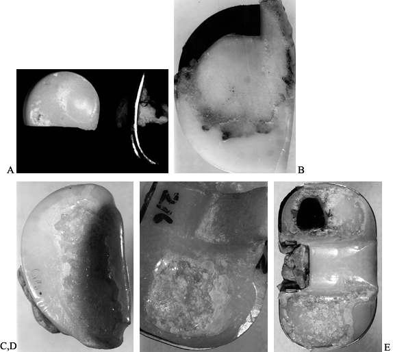 |
|
Figure 100.53. Examples of wear on different TKR designs with different types of polyethylene: abrasive wear (A), adhesive wear (B), deformation (C, D), and delamination (E) can all be seen.
|
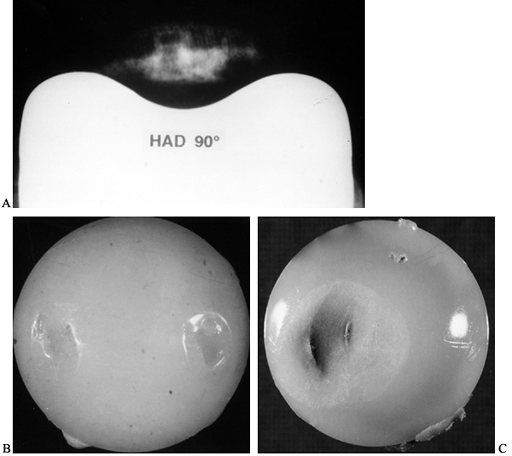 |
|
Figure 100.54.
An anatomically shaped patella is ideal for a retained patella. When a dome is used, however, deformation can readily occur, as in these examples. |
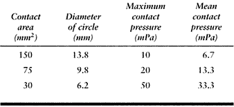 |
|
Table
100.4. Contact Areas (Diameters of Circular Areas Are Given) and Contact Pressures, Covering the Range for Condylar Replacement Knees in Extension and Flexion |
In knees of low conformity, as the femur slides over the plastic
surface, a deformed groove up to 0.3 mm deep occurs in the first
few
months of use, and thereafter the groove is steadily deepened by wear.
In knees of moderate to high conformity, the deformed area is
relatively small, with a depth of less than 0.1 mm. Within the contact
area, there are a multitude of local contact points at a micron level,
depending on the microroughness of both the metal and plastic surfaces.
There are several mechanisms whereby small particles are released. Some
of these mechanisms are fatigue processes requiring numerous cycles of
sliding. Multidirectional sliding is also more damaging than sliding,
which is predominantly limited to the same direction. The wear
processes also depend on whether the kinematics involve rolling,
tractive rolling, or sliding (23,28). These wear processes (27,60,61) are as follows:
-
Adhesive wear occurs when the local
frictional shear force on transverse ripples or asperities of
polyethylene causes shear deformation or stretching of a fibril. The
fibrils are typically 2 to 5 µm in length and 0.2 to 0.5 µm in diameter. -
A third form of adhesive wear occurs when
a surface layer about 0.1 to 0.2 µm in thickness becomes sheared with
respect to the underlying material, similar to the formation of a
blister. Eventually, the layer fragments to form flakes approximately 2
to 10 µm across. -
A small scratch on the metal surface with
ridges will produce direct cutting or ploughing into the plastic.
Several passes across a groove in the plastic, especially at angles to
previous passes, will release fibrils or granules of polyethylene. This
is called two-body abrasive wear -
If hard particles become entrapped in the
contact area, they will also cut grooves in the plastic, causing wear
called three-body abrasive wear. Plastic particles themselves can
produce this type of wear, but to a much lesser extent than hard
particles such as metal, ceramic, or bone.
Ripples perpendicular to the sliding direction are typical. Fibrils are
seen to be stretched from the crests of the ripples, while there is
also evidence of granule formation. Shearing of the surface layer
results in fibrils or thin flakes. Fluid samples, after processing, can
be filtered to show the resulting particles. They are categorized into granules, fibrils, and flakes (47,48).
The types and sizes of particles are indicative of the wear mechanisms
that were taking place. In general, smaller particles produce more
expression of cytokines from cells.
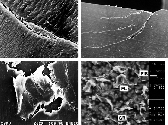 |
|
Figure 100.55. Scanning electron micrographs of retrieved plastic components. Top left: Ripples transverse to the sliding direction with fibrils and granules being formed on the crests of the ripples. Top right: Cracks shown in a section perpendicular to the surface, which coalesce to produce delamination. Bottom left: Shearing of a thin surface layer producing flakes. Bottom right: Processed and filtered fluid samples show wear particles of three types: GR, granules; FIB, fibrils; FL, flakes.
|
surface of the plastic. However, other wear mechanisms are more
appropriately called “damage mechanisms.” These mechanisms involve more
general breakdown of the surface region of the material, including
failure that starts entirely subsurface (205).
These damage mechanisms, and other phenomena that involve cracks at and
under the surface, are dependent on the component geometry, the sliding
conditions, and the type of UHMWPE (81,189,190). To illustrate this point, a typical contact situation is shown in Figure 100.56.
Around the periphery of the contact area, radial tensile stresses occur
of magnitude 0.13 times the maximum compressive stress (124).
As sliding and rolling take place, at a particular location on the
plastic surface, the stresses cycle between tensile and compressive.
This is equivalent to the stresses in a bar of material subject to
repeated bending in opposite directions. As a result, cracks will be
produced on the surface, which will progress along the surface and into
the material, but because the tensile stresses reduce with depth, the
crack depth is limited. However, when the cracks are not perpendicular
to the surface and adjacent cracks coalesce, pits are formed with
typical dimensions of 0.5 to 2 mm in width and depth. Such pits are
commonly seen on retrieved components (18,63,139), from low to high conformities (27), including mobile bearings.
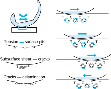 |
|
Figure 100.56.
As the femoral component slides and rolls across the surface, the surface stresses cycle between tension and compression, and the subsurface shear stresses change in direction. These cyclic stresses, representing a fatigue process, produce cracks, pits, and delamination. |
propagate beneath the surface. This is termed “delamination.” A typical
crack depth is 1 mm, and the initial area affected can be several
millimeters across, seen as a white patch (18,27,29).
These cracks are associated with regions of maximum shear stress, which
occur beneath the center of a contact area at a depth of approximately
0.25 times the contact width, usually 1 to 2 mm. The direction of the
maximum shear stress is at 45° to the surface (Fig. 100.56).
Beneath the periphery of the contact area in the cross-sectional plane,
there are further peaks of shear stress of lesser magnitude oriented at
90° to the surface. The stress directions are opposite at the leading
and trailing edges of the contact area. Hence, as the femoral component
slides across the plastic, particular points beneath the plastic
surface experience shear stresses that change in direction, producing a
fatigue situation that leads to crack formation. Once the cracks reach
the surface, the consequent disruption of the surface leads to rapid
delamination of adjacent areas, eventually covering the entire contact
region. Examples are shown in Figure 100.53 and in sectional view in Figure 100.55.
This is based on the assumption that the amount of wear at the surface
(adhesive and abrasive wear) and damage within the material (pitting
and delamination) are inversely proportional to the contact area or
proportional to the contact pressure. There are some data in the
literature to support this, based on the testing of specimens in wear
test machines, and there is the general impression from retrievals that
the wear is more severe in designs with small contact areas, usually
cruciate-retaining designs. There is, however, the question as to which
angle or angles of flexion should be used to measure the contact area.
If the majority of wear is assumed to occur during the stance phase of
walking, then areas measured between about 0° and 15° of flexion are
relevant. Depending on the posterior-distal transition angle (Fig. 100.40),
these areas can differ considerably. There is also the possibility that
severe wear occurs at the less frequent activities, which generate
higher forces at higher flexion angles. Hence, the use of area of
contact as a measure should include values for a range of flexion
angles. A weakness of using contact area alone is that it does not
account for sliding distance.
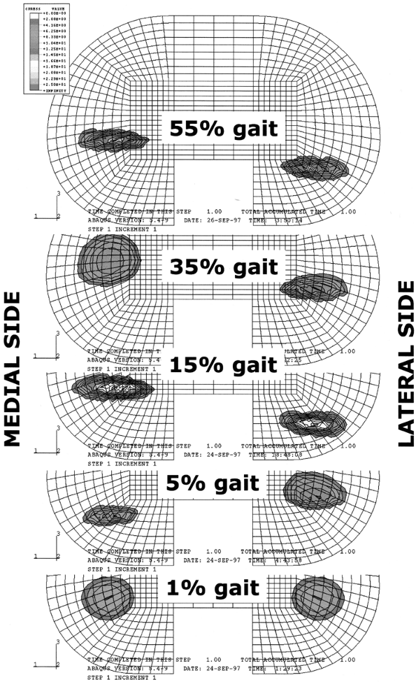 |
|
Figure 100.57.
The locations of the contact areas and the contact stresses calculated using finite element analysis, at different times in the gait cycle (191). The calculations took into consideration the forces and moments (including torque) between the femur and the tibia, the geometries of the femoral and tibial bearing surfaces in the contact region, and the frictional shear forces. |
pitting and delamination. If it is assumed that the wear factor and
load are the same for all TKRs, then the wear is proportional to the
sliding distance, which is related to the femoral and tibial radii in
the sagittal plane, in other words, the inherent constraint. Hence a
simple indicator for wear is the AP sliding distance of the contact
points (not the relative rigid body motion itself) for a typical
activity cycle. For purposes of comparison between different TKRs, the
sliding distance can be determined based on the data for walking and
other activities, which shows that, in stance, along with an axial
compressive force, there are both anterior and posterior shear forces.
This can be simplified, as shown in Figure 100.58,
by applying the compressive force first, followed by the anterior and
posterior shear forces. As determined by the triangle of forces, the
point of equilibrium is reached at a particular angle θ on the plastic
surface. This point is entirely dependent on the tibial radius and not
the femoral radius, and can be calculated directly from the tibial
dimensions. If the tibial articular geometry is shallow, so that the
slope cannot be reached, the displacement limit would be from soft
tissues, at an assumed distance of approximately 12 mm from neutral.
The sliding distance is the distance between the anterior and posterior
points. Although this test accounts for sliding distance, it does not
account for the effect of contact pressure on the wear factor.
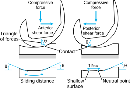 |
|
Figure 100.58.
A proposed measure for estimating the surface wear in a TKR where a cyclic shear force is applied and the sliding distance is used as a measure of the wear. The distance can be obtained directly from engineering drawings of the tibial component, using simple geometry: tan θ = shear force/compressive force.. |
method involving all aspects of the TKR geometry, as well as the forces
and motions in activity. The following damage function model describes
such a method.
However, the surface wear can easily be included, as will be explained
later. As already described, delamination is due to the initiation and
propagation of subsurface cracks in the polyethylene. The likelihood of
a crack developing and the rate of crack propagation can be described
by the strain energy input to an element of material during a complete
activity cycle. Calculation of this parameter has been carried out as
follows:
-
Specify the input forces, moments, and flexion angles on the knee during activity, and divide this into equal time increments.
-
Use specially written software (a
kinematic solver) to determine successive contact point locations on
the lateral and medial sides, at each increment, taking surface
friction into account (188) (Fig. 100.57). -
Use FEA to calculate the subsurface shear
stresses at a multitude of quadrilateral elements below the surface of
the plastic at each increment. -
For each element, plot a shear-stress versus time curve.
-
By treating this in a manner similar to a
force displacement curve, the shear strain energy can be calculated for
each element as the areas under the curve. -
Plot the shear strain energy, called the damage function, for the elements at different subsurface levels.
This plot shows a comparison between knees of different frontal and
sagittal geometries, demonstating the regions of plastic most likely to
generate cracks, and predicts the relative susceptibilities of the
different knees to delamination wear.
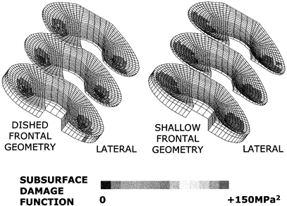 |
|
Figure 100.59.
Plots of the damage function for elements of plastic at different levels below the surface for condylar knees of different geometries (Fig. 100.40). High susceptibility to delamination (left) is predicted for small frontal femoral radius, high frontal femorotibial clearance, and small PDTA. At the other extreme of condylar geometry, delamination is predicted to be low (right). Also, the large frontal radius allows for adequate rotational laxity. (From Robinson R, Clark JE. Uncemented press-fit total hip arthroplasty using the identifit custom-molding technique. J Arthroplasty 1995;11:247.) |
also be calculated. The method would be to use the basic wear equation
for the incremental steps used in calculating the contact areas (Fig. 100.57).
The wear in each increment would be the average load acting times the
sliding distance. The wear factor could also be expressed as a function
of the contact pressure. However, at this time, reliable data are not
available.
effect both on surface wear and on subsurface delamination. This has
been discussed already in relation to hips, but there are a number of
factors specifically related to knees. When retrieved tibial components
are sectioned, the region of highest oxidation is typically 1 to 2 mm
beneath the surface, although the zone can extend completely to the
surface (18). It is noticeable that oxidation
is highest beneath the contact areas, indicating a relation with fluid
transport and local stress fluctuations. Such oxidation increases the
density and the elastic modulus, and decreases the tensile strength,
elongation to break, and toughness. All of these factors make the
plastic more susceptible to delamination. Newer processing methods,
which reduce oxidation are likely to extend the durability of UHMWPE
before delamination occurs (18).
that the use of directly molded polyethylene, even in designs of low
conformity, avoids delamination almost completely, although surface
wear from adhesion and abrasion is still observed (27,29). It is possible that such material is resistant to oxidation and degradation of mechanical properties.
than from the bearing surfaces. “Back-side wear” between the plastic
and the metal tray occurs due to micromotion at that interface. Snap-in
capture mechanisms, combined with the manufacturing tolerances, can
result in considerable motion under shear and torque, even up to 1 mm.
If this is accompanied by a rough surface in the metal tray, severe
wear can occur. The effects of such wear have been noted particularly
in trays with holes for fixation screws, around which osteolytic
lesions have developed.
simplifications of reality that embody sufficient and appropriate
characteristics of the actual situation to address the question being
asked. In some cases, simple tests suffice; in other cases, a complex
test is required.
relations and the forces within the knee is to mount the tibia on a
base, apply a flexion moment to the femur, and balance the knee at a
particular angle using a turnbuckle in the quadriceps. The original
apparatus was termed the Oxford rig (97), but the design has since evolved (240) (Fig. 100.60). Aspects that have been studied using such a rig include:
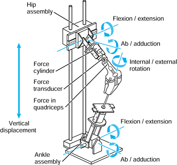 |
|
Figure 100.60.
An Oxford-type static loading test rig for studying the basic mechanics of the knee. The rig allows the full 6 degrees-of-freedom motion of the knee. A downward force at the hip is balanced by a force in a cable representing the quadriceps (240). |
-
The femorotibial contact point or area locations (111), determined radiographically or using pressure-sensitive film inside the knee.
-
The orientation of and forces in the
ligaments; the forces have been measured by small turnbuckles or by
dissociation of bone blocks. -
The force in the quadriceps and in the patellar tendon using force transducers
-
The patellofemoral contact areas and pressures, and the effect of different relative forces in the components of the quadriceps.
the fact that the force may not simulate the direction of the external
force at the knee in the frontal and sagittal planes, and only one
muscle being represented. Such factors can be addressed in more
sophisticated versions of the rig. An extreme example is the use of a
robot to position the femur on the tibia in a known 3-D orientation,
which can then be used to study the contributions of different
structures to resisting applied forces and moments.
wear before it is used in patients. In general, the tests should be
carried out on the standard-sized components. The test should replicate
as far as possible the physiologic conditions while maintaining
mechanical simplicity. The
rate of testing can be up to 5 Hz for metal components and up to 2 Hz where plastic is involved.
The adverse design factors have been internal corners, notches, a thin
plate, and grooves or coatings. The clinical factors have been patient
weight and activity level, and loss of bony support under one condyle.
The test proposed by the ISO involves clamping one half of the
component and then applying a cyclic force to the unsupported condyle (Fig. 100.61).
The test does not reproduce the changing contact point locations during
function. Furthermore, it has been found that an appropriate force for
testing is around 500 N, whereas forces at physiologic levels in
walking of 2000 N or more (or even half this value for one-condyle
loading) would cause most existing baseplates to fail in fatigue. In
this sense, the test is an exaggeration of reality. A typical number of
cycles for such tests is 10 million, although this would represent only
5 to 7 years of use in most patients.
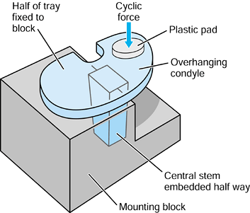 |
|
Figure 100.61.
The ISO test for mechanical strength of tibial trays. A finite element model can be used to predict the failure location (From Ahir SP, Blunn GW, Haider H Walker PS. Evaluation of a testing method for the fatigue performance of total knee tibial trays. J Biomech 1999;2:1049.) |
security of fixation of the plastic in the metal tray, and the security
of mobile bearing components can be tested using an applied cyclic
shear force, possibly accompanied by a compressive force (Fig. 100.62).
From a compilation of available force data in the knee, including that
from a telemetrized distal femoral replacement, a suitable cyclic shear
force is 750 N applied for 10 million cycles, interspersed with a force
of 1250 N applied for a total of 0.5 million cycles. The former
represents vigorous walking, and the latter represents the extreme
forces that could be applied in rapid ascending or descending. In the
opposite direction (such that the ACL would be tensed) suitable values
are 500 and 750 N.
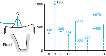 |
|
Figure 100.62. Testing knee components in shear (S) with a compressive force (C) applied. Values of S in direction shown under different conditions: A: level walking (157); B: ascending (156); C: level walking (206); D: level walking (Andriacchi 1998, personal communication); E: TKR dislocation forces (Greenwald 1993, internal report, Cleveland Clinic, Cleveland, OH); F: TKR dislocation (144); G, H: TKR 5 mm from dislocation (188).
|
This can be accomplished using a cyclic force that is offset from the
centerline and medial to the medial femorotibial contact point. For
comparative testing applicable to all designs, the offset distance from
the center of the knee and the
applied
force should be the same. A normal value of the external moment acting
at the knee during activity is 3% BW times height, whereas an extreme
value is 6.5% BW times height (159). To determine a suitable test force, consider a value of the external varus moment of 5% × BW × height = 67,500 N·mm for a typical man. The moment carried by the reaction force of 3 BW on the medial condyle at 22 mm spacing = 44,550 N·mm. Hence, the moment carried by the central post is 22,950 N·mm.
This can be applied by a force of C = 1000 N acting at 23 mm from the
contact point or 45 mm from the center of the knee. In such a test,
superstabilizers with plastic posts show considerable progressive
angular deformation, which is reduced but not eliminated by metal
reinforcement. Fixed or rotating hinges show only small deformations.
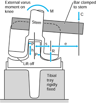 |
|
Figure 100.63. Testing superstabilizers and similar designs in varus. The total moment M is equilibrated by R × s and by P × h. The moment P × h is produced by C × e, C being the cyclic test force.
|
complex knee simulator could be used. However, a uniaxial cyclic load
machine can be used to apply multiaxial forces and moments. This is
achieved by mounting the component at an angle and applying the force
offset (Fig. 100.64). In this way, the following is applied by the single uniaxial force:
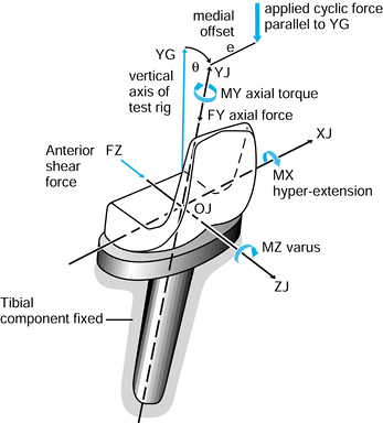 |
|
Figure 100.64. If a total knee is extended by θ and a single force offset by e
is applied relative to the TKR axes, simultaneous force components and moments occur. This exerts a rigorous test condition on the device. |
-
Compressive force.
-
AP shear force.
-
Varus moment.
-
Hyperextension moment
-
Axial torque.
in a design not shown by simpler testing, as well as effectively
applying several test modes simultaneously.
measuring wear and deformation in TKRs. If the primary concern is to
compare a new plastic or a new metal surface, a pin-on-plate test is
appropriate (Fig. 100.65). To produce a model
that is simple but a close model to the actual TKR, a metal pin with a
spherical surface at the end (femoral) is slid to-and-fro on a flat
plastic plate (tibial) (216). To account for
internal-external rotation, the pin is rotated cyclically about its own
axis. The surrounding medium is 25% to 50% serum at 37°C. The fluid
requires changing every 2 days to minimize degradation. The sliding
distance is a total of 10 mm. The radius of the spherical end should
produce a similar relative radius of curvature to the TKR design
envisaged. A static load of 1000 N is applied, representing one
condyle. Samples of fluid are collected every million cycles for
particle analysis. A suitable characterization is to divide particles
into granules, fibrils, and flakes, and measure the size ranges and the
percentages of each (47,48).
The rate of testing is limited to 1 Hz (2 Hz maximum) to avoid
overheating at the contact. It is observed that in the first few
hundred thousand cycles, deformation of the plastic predominates over
wear, whereas as the contact pressure thereby reduces, deformation
reduces and
wear
predominates. If the objective of a test is to determine the effect of
load, contact area, or contact pressure on wear, the above-mentioned
configuration can be reversed with a flat-ended plastic pin sliding on
a flat metal plate.
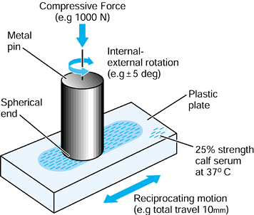 |
|
Figure 100.65.
A simple test for simulating the bearing conditions of a TKR to assess new materials or surfaces. The motion is a combination of sliding and rotation. |
load and motion cycles are applied to an actual TKR, a knee simulator
is required (40,217).
If the goals of the design of a simulator are simplicity, low cost,
reliability, and ease of use, then this would result in a machine that
applies a constant compression force, only in flexion-extension.
However, such a machine does not satisfy the criterion for a close
simulation of reality, as previously described for hip Simulators. The
input required is replication of a walking cycle, preferably with 5% to
10% of more rigorous inputs representing ascending and descending. This
involves the following cyclic inputs:
-
Compressive force.
-
Varus moment.
-
AP shear force.
-
Internal-external torque
-
Flexion-extension.
moments acting across the knee are independent of the type of TKR, no
matter what the constraint. This leads to a concept for a knee
simulator design called force input (217) (Fig. 100.66).
In the test setup, the relative motions between the femur and tibia,
except flexion-extension, are unconstrained. However, mechanical
springs are mounted between the femoral and tibial holders, to simulate
soft-tissue restraint. Although the input force data from the
literature have been obtained by indirect means and are therefore
uncertain, and accounting for the variations between individuals,
estimates of the inputs can be specified to provide a reasonable
representation of normal activity. Measurements of the output
displacements and rotations show that the patterns are highly dependent
on the constraints of the particular TKRs. In turn, the wear will
depend on the displacements and rotations, and hence the force-input
concept seems justified.
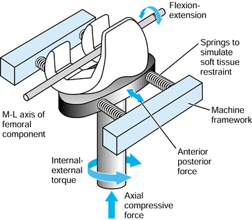 |
|
Figure 100.66.
Schematic of the force-input concept of a knee simulator design. The movement of each knee depends on its inherent constraint, with the springs representing soft-tissue restraint and preventing excessive movements. |
mechanically, is a displacement-input machine to which AP displacement
and internal-external rotation are applied rather than force and torque
(40). For the force-input approach, each knee
moves according to its inherent constraint, and therefore, comparative
testing would seem valid. For displacement-input, however, a means of
specifying the input displacements for each individual knee is
required. This could be achieved by using a simple test rig initially.
However, fixed displacements and rotations would not allow for changes
that might occur over time due to deformation and wear.
forces, together with forces in the quadriceps and possibly other
muscles. There would be some similarity with the scheme shown in Figure 100.60.
To produce a dynamic version, however, there would be increased
mechanical complexity and high demands on the control systems, but the
overall scheme is more realistic and the patellofemoral joint can be
tested simultaneously (personal communication: B.M. Hillberry, Perdue
University).
particular knee design need to be compared with tests of an earlier
design with known clinical history. Furthermore, the duration of the
testing needs to be sufficient (153,195), at
least 5 million cycles, to account for early bedding in, fatigue phenomena, and possible material degradation.
have contributed indirectly to this chapter. Thanks are especially due
to the staff and associates of the Center for Biomedical Engineering
(Faculty of Clinical Sciences, and Department of Mechanical
Engineering, University College London), located at the Royal National
Orthopaedic Hospital Trust, Stanmore, near London, UK.
scheme: *, classic article; #, review article; !, basic research
article; and +, clinical results/outcome study.
AM, Burke DL, Yu, A. In-vitro Measurement of Static Pressure
Distribution in Synovial Joints—Part II: Retropatellar Surface. Transactions of the American Society of Mechanical Engineers 1983;105:226.
WT, Callaghan JJ, Sullivan PM, Johnston RC. The Results of Improved
Cementing Techniques for Total Hip Arthroplasty in Patients Less Than
Fifty Years Old. J Bone Joint Surg 1994;76-A:959.
DL, Bicknell VL, Wright TM. The Effect of Conformity, Thickness and
Material on Stresses in Ultra High Molecular Weight Components for
Total Joint Replacement. J Bone Joint Surg 1986;68-A:1041.
GS, Vasu R, Carter DR, Schurman DJ. Epiphyseal Based Designs for Tibial
Plateau Components—II. Stress Analysis in the Sagittal Plane. J Biomech 1986;19:663.
C, Walker PS, Abeysundera M, et al. Effect of Oxidation on Delamination
of Ultra-high-molecular-weight Polyethylene Tibial Components. J Arthroplasty 1998;13:280.
V, Hahn GT, Rubin CA. An Elastic-plastic Finite Element Model of
Rolling Contact. Part 2—Analysis of Repeated Contacts. J Appl Mech 1984;84-WA/APM-43:9.
GW, Joshi AB, Lilley PA, et al. Polyethylene Wear in Unicondylar Knee
Prostheses: 106 Retrieved Marmor, PCA and St. Georg Tibial Components
Compared. Acta Orthop Scand 1992;63:247.
P, Walch G. The Three-dimensional Geometry of the Proximal Humerus.
Implications for Surgical Technique and Prosthetic Design. J Bone Joint Surg 1997;79-B:857.
FF, Pappas MJ. Long-term Survivorship Analysis of Cruciate-sparing
Versus Cruciate-sacrificing Knee Prostheses Using Meniscal Bearings. Clin Orthop 1990;260:162.
WD, Culpepper WJ, Engh CA Jr, Engh CA Sr. Long-term Clinical
Consequences of Stress-shielding After Total Hip Arthroplasty without
Cement. J Bone Joint Surg 1997;79-A:1007.
P, van Loon PJM, Versleyen H, et al. Histological and Biomechanical
Analysis of Bone and Interface Reactions Around Hydroxyapatite-coated
Intramedullary Implants of Different Stiffness: A Pilot Study on the
Goat. Biomaterials 1997;18:1251.
DL, Kay MD, Stouffer DC. Comparison of Material Properties in
Fascicle-bone Units from Human Patellar Tendon and Knee Ligaments. J Biomech 1986;19:425.
DLA, Hopper RH, Lin GM, Myers BS. An Improved Method for Finite Element
Mesh Generation of Geometrically Complex Structures with Application to
the Skullbase. J Biomech 1997;30:1067.
L, Dowson D, Fisher J, Jobbins B. The Influence of Bone and Bone Cement
Debris on Counterface Roughness in Sliding Wear Tests of Ultra-high
Molecular Weight Polyethylene on Stainless Steel. Proc Inst Mech Eng [H] 1990;204:65.
LV, Albrektsson BEJ, Freeman MAR, et al. A New Radiographic Method for
Detection of Tibial Component Migration in Total Knee Arthroplasty. J Arthroplasty 1993;8:117.
EY, Laughman RK, Schneider E, Stauffer RN. Normative Data of Knee
Motion and Ground Reaction Forces in Adult Level Walking. J Biomechanics 1983;16:219.
SL, Davey JR, Inman RD, et al. The Effect of the Medial Collar in Total
Hip Arthroplasty with Porous-coated Components Inserted Without Cement.
J Bone Joint Surg 1995;77-A:118.
K, Kuhn JL, Ciarelli MJ, Goldstein SA. The Elastic Moduli of Human
Subchondral Trabecular and Cortical Bone Tissue and the Size-dependency
of Cortical Bone Modulus. J Biomech 1990;23:1103.
JP, Mayor MB, McNamara JL, et al. Analysis of the Failure of 122
Polyethylene Inserts from Uncemented Tibial Knee Components. Clin Orthop 1991;273:232.
JA. Characteristics of Metal and Ceramic Total Hip Bearing Surfaces and
Their Effect on Long-term Ultra High Molecular Weight Polyethylene
Wear. Clin Orthop 1993;294:361.
PA, Robinson EJ, Bourne RB, et al. Measurement of Polyethylene Wear in
Acetabular Components Inserted with and without Cement. J Bone Joint Surg 1997;79-A:682.
KE, Wright TM, Rimnac CM, et al. Fatigue Crack Propagation Behaviour of
Ultra High Molecular Weight Polyethylene Under Mixed Mode Conditions. J Biomed Mater Res 1994;28:181.
J, Firkins P, Reeves EA, et al. The Influence of Scratches to Metallic
Counterfaces on the Wear of Ultra-high Molecular Weight Polyethylene. Proc Inst Mech Eng [H] 1995;209:263.
MAR, Railton GT. Should the Posterior Cruciate Ligament Be Restrained
or Resected in Condylar Nonmeniscal Knee Arthroplasty? The Case for
Resection. J Arthroplasty 1988;3:S3.
T, Torzilli PA, Sherman MF, Warren RF. An In Vitro Biomechanical
Evaluation of Anterior-posterior Motion of the Knee. Tibial
Displacement, Rotation, and Torque. J Bone Joint Surg 1982;64-A:258.
ES, Suntay WJ. A Joint Co-ordinate System for the Clinical Description
of Three-dimensional Motions: Application to the Knee. J Biomech Eng 1983;105:136.
ML, Harding L, Goodfellow JW. A Preliminary Report of a Simple Rig to
Aid Study of the Functional Anatomy of the Cadaver Human Knee Joint. J Biomech 1977;10:517.
WH, Mulroy RD, Maloney WJ, et al. Intraoperative Measurements of
Rotational Stability of Femoral Components of Total Hip Arthroplasty. Clin Orthop 1991;266:119.
DT, Sidles JA, Harris SL, et al. The Effect of Articular Conformity and
the Size of the Humeral Head Component on Laxity and Motion After
Glenohumeral Arthroplasty. J Bone Joint Surg 1995;77-A:555.
DA, Marmor L, Gibson A, Rougraff BT. Unicompartmental Knee
Arthroplasty. A Multicenter Investigation with Long-term Follow-up
Evaluation. Clin Orthop 1993;286:154.
MS, Yang H. A Three-dimensional Anatomical Model of the Human
Patello-femoral Joint, for the Determination of Patello-femoral Motions
and Contact Characteristics. J Biomed Eng 1993;15:289.
K, Bauer TW, Stulberg BN, et al. Characterization and Comparison of
Wear Debris from Failed Total Hip Implants of Different Types. J Bone Joint Surg 1996;78-A:1235.
J, Walker PS. Relative Motion of Hip Stems Under Load: An In Vitro
Study of Symmetrical, Asymmetrical and Custom Asymmetrical Designs. J Bone Joint Surg 1994;76-A:95.
OL, Bansal M, Betts F, et al. Polyethylene and Metal Debris Generated
by Non-articulating Surfaces of Modular Acetabular Components. J Bone Joint Surg 1994;76-B:568.
JN. Historical Development, Classification and Characteristics of Knee
Prostheses. In: Insall JN, Windsor RE, Scott WN, et al., eds. Surgery of the Knee, 2nd ed. New York: Churchill Livingstone, 1993:677.
M, O’Connor DO, Henshaw RM, et al. Fit of the Uncemented Femoral
Component and the Use of Cement Influence the Strain Transfer to the
Femoral Cortex. J Orthop Res 1994;12:648.
RC, Moines D, Fitzgerald RH, et al. Clinical and Radiographic
Evaluation of Total Hip Replacement. A Standard System of Terminology
for Reporting Results. J Bone Joint Surg 1990;72-A:161.
TJ, Unsworth A. A Comparison of the Wear of Cross-linked Polyethylene
Against Itself with the Wear of Ultra-high Molecular Weight
Polyethylene Against Itself. Proc Inst Mech Eng [H] 1996;210:297.
SM, Rimnac CM, Santner TJ, Bartel DL. Exponential Model for the Tensile
True Stress-strain Behavior of As-irradiated and Oxidatively Degraded
Ultra High Molecular Weight Polyethylene. J Orthop Res 1996;14:755.
PF, Falatyn SP. Clinical and Radiographic Results of the Total Condylar
III and Constrained Condylar Total Knee Arthroplasty. J Arthroplasty 1996;11:916.
JR, Dorey F, Shekelle P, et al. Differences Between Patients’ and
Physicians’ Evaluations of Outcome After Total Hip Arthroplasty. J Bone Joint Surg 1996;78-A:835.
E, Sathasivam S, Walker PS. Inherent Differences in the Laxity and
Stability Between the Intact Knee and Total Knee Replacements. The Knee 1997;4:7.
TA, Brown TD, Pedersen DR, Callaghan JJ. A Sliding-distance-coupled
Finite Element Formulation for Polyethylene Wear in Total Hip
Arthroplasty. J Biomech 1996;29:687.
BJ, Shinar AA, Freiberg AA, Harris WH. Enhancement of the Value of Hip
Questionnaires by Telephone Follow-up Evaluation. J Arthroplasty 1997;12:340.
JC, Mulier M, Brady LP, et al. A New System to Produce Intraoperatively
Custom Femoral Prosthesis from Measurements Taken During the Surgical
Procedure. Clin Orthop 1989;249:97.
SJ, Kras TJ, Mallory TH. Empirical Considerations in Orthopaedic
Research Design and Data Analysis. Part III: Multivariable Analysis. J Arthroplasty 1990;5:111.
KG, Karrholm J, Ekelund L, Magnusson P. Evaluation of Micromotion in
Cemented vs Uncemented Knee Arthroplasty in Osteoarthrosis and
Rheumatoid Arthritis. J Arthroplasty 1991;6:265.
MH, Jakob RP, Schneider E, Hoogewoud H-M. Radiological Analysis of
Normal Axial Alignment of Femur and Tibia in View of Total Knee
Arthroplasty. J Arthroplasty 1993;8:419.
L, Koo J, Rimnac CM, et al. Cyclic Compressive Loading Results in
Fatigue Cracks in Ultra High Molecular Weight Polyethylene. J Orthop Res 1995;13:143.
PJ, Rakotamanana RL, Leyvraz PF, et al. Frictional Interface
Micromotions and Anisotropic Stress Distribution in a Femoral Total Hip
Component. J Biomech 1993;26:725.
TP, Kwong LM, Jasty M, et al. The Mechanism of Loosening of Cemented
Acetabular Components in Total Hip Arthroplasty. Clin Orthop 1992;274:60.
DF, Jaffe WL. Host-bone Response to Porous-coated Cobalt-chrome and
Hydroxyapatite-coated Titanium Femoral Components in Hip Arthroplasty. J Arthroplasty 1996;11:429.
H, Bechtold JE, Sherman RE, Gustilo RB. Stability of Initial Fixation
of the Tibial Component in Cementless Total Knee Arthroplasty. J Orthop Res 1990;8:64.
A, Danmak M, Forcione A, Paiement G. Friction Measurements at the
Bone/Implant Interface—Application to Analysis of Cementless
Prostheses. Trans Orthop Res Soc 1992;17:382.
HB, Kilgus DJ, Keyak J, et al. Correlation of Computed Finite Element
Stresses to Bone Density after Remodeling Around Cementless Femoral
Implants. Clin Orthop 1994;305:178.
RC, Barbagallo S, Slater GL, et al. Measurement of Periprosthetic Bone
Density in Hip Arthroplasty Using Dual-energy X-ray Absorptiometry. J Arthroplasty 1996;11:445.
JB, Komistek RD, Dennis DA, et al. Fluoroscopic Analysis of Kinematics
after Posteriorcruciate Retaining Knee Arthroplasty. J Bone Joint Surg 1995;77-B:884.
S, Walker PS, Perry J, et al. The Forces in the Distal Femur and the
Knee During Walking and Other Activities Measured by Telemetry. J Arthroplasty 1998;13:428.
Lenthe H, De Waal Malefijt M, Huiskes R. Bone Resorption in the Distal
Femur After Total Knee Arthroplasty Can Be Caused by Stress Shielding. J Bone Joint Surg 1997;79-B:117.
PS, Unsworth A, Dowson D, et al. Mode of Aggregation of Hyaluronic Acid
Protein Complex on the Surface of Articular Cartilage. Ann Rheum Dis 1970;29:591.
H, Huiskes R, van Rietbergen B, et al. Adaptive Bone Remodeling Around
Bonded Noncemented THA: A Comparison Between Animal Experiments and
Computer Simulations. J Orthop Res 1993;11:500.
JN, Andriacchi TP, Galante JO. Factors Influencing Walking and
Stairclimbing Following Unicompartmental Knee Arthroplasty. J Arthroplasty 1986;1:109.
LA, Arima J, White SE, et al. Fixation of the Modular Total Hip Femoral
Component in Cementless Total Hip Arthroplasty. Clin Orthop 1994;298:184.
BM, Siney PD, Dowson D, Collins SN. Prospective Clinical and Joint
Simulator Studies of a New Total Hip Arthroplasty Using Alumina Ceramic
Heads and Cross-linked Polyethylene Cups. J Bone Joint Surg 1996;78-B:280.