
II – FRACTURES, DISLOCATIONS, NONUNIONS, AND MALUNIONS > Malunions
and Nonunions > CHAPTER 32 – MANAGEMENT OF FRACTURES, NONUNIONS, AND
MALUNIONS WITH ILIZAROV TECHNIQUES
Pediatric Orthopaedics, Arkansas Children’s Hospital; Department of
Orthopaedics, University of Arkansas for Medical Sciences, Little Rock,
Arkansas, 72202.
A. Green was editor of a seven-chapter section on ring fixation and
distraction techniques. To eliminate repetition and to provide a more
coordinated presentation of the techniques developed by Professor G. A.
Ilizarov, Dr. Green has reedited and consolidated the first five of
those chapters, which now appear in this chapter as five parts. Much of
the original material, both text and illustrations, has been retained,
and we thank Drs. James Aronson, Dror Paley, Kevin D. Tetsworth, and J.
Charles Taylor for their superb contributions to those second-edition
chapters. Deborah F. Stanitski has consolidated the two second-edition
chapters on pediatric applications into the new Chapter 171, located in Section IX.
unlimited quantities of living bone directly from a special osteotomy
by controlled mechanical distraction. The new bone spontaneously
bridges the gap and rapidly remodels to a normal macrostructure for the
local bone (1,2,13,14 and 15).
Ilizarov in Kurgan, Siberia, since he first observed this process in
one of his patients in about 1956 (8). Using
ring external fixators and small-diameter (1.5–1.8 mm) wires under
tension, Ilizarov has regenerated more than 18 cm of new bone from a
single operative intervention, often doubling the baseline bone length (15,19).
formation in any plane, as the distraction osteogenesis always follows
the vector of applied force (13,14).
Age is not a limitation so long as the patient has the potential to
heal a fracture. The indications for this surgical technique are
similar to those for traditional bone grafting and include limb
lengthening, nonunions, pseudarthroses, and any osseous defect from
trauma, tumor, or infection (12).
completely vital bone, capable of bearing load, at about 1 cm of bone
length per month in children, and 1 cm per 2 months in adults (10,11,18,19).
osteogenesis. By varying the stability of fixation, the energy of the
osteotomy (i.e., the degree of vascular damage), and the rate and the
rhythm of distraction, he has postulated that all four factors are
critical to osteogenesis (13,14).
means new bone production between vascularized bone surfaces, separated
by gradual distraction. Most commonly, the bone is separated by a
corticotomy and then distracted at a rate of 1 mm per day (divided into
a rhythm of 0.25 mm four times per day) following a 5-day or longer
latency.
time after a corticotomy when the initial healing response bridges the
cut bone surfaces, before initiating distraction.
means the conversion of nonosseous interpositions (e.g., fibrocartilage
in nonunions, synovial cavities in pseudarthroses, or muscle in delayed
unions) into normal bone by combined compres and distraction forces,
sometimes augmented by a nearby corticotomy.
latency period appears to be no different from routine fracture
healing, as might be expected. Fibrin-enclosed hematoma and
inflammatory cell infiltration fill the gap at the corticotomy site. At
the start of distraction, mesenchymal cells begin to organize a bridge
of collagen and immature vascular sinusoids.
organize itself parallel to the direction of distraction. The collagen
network becomes more dense and less vascular, almost resembling tendon,
while the vascular channels remain at the edges closely approximated to
the cut surfaces of the corticotomy segments (1,2,3,5,6 and 7).
of relatively avascular fibrous tissue bridges the entire 6- to 7-mm
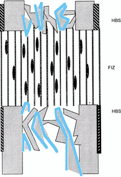
gap, which is called the fibrous interzone (FIZ). Spindle-shaped cells
resembling fibroblasts are loosely interspersed between collagen
bundles; neither osteoid nor osteoblasts are present (Fig. 32.1). Bone mineral is distinctly absent (1,2,3,5,6 and 7).
 |
|
Figure 32.1.
Distraction osteogenesis, week 1. Spindle-shaped fibroblasts are interspersed among parallel bundles of collagen that bridge the two cut bone surfaces. This bridge covers the entire host bone surface (HBS), including periosteum, cortex, and cancellous bone in the medullary canal. The majority of blood vessels are located in the intramedullary region but do not cross the fibrous interzone (FIZ). |
cells appear in clusters adjacent to the vascular sinuses on either
side of the FIZ. Collagen bundles become fused with a matrix resembling
osteoid. The osteoblastic cells initially rest on the surface of these
primary bone spicules and eventually become enveloped within, as the
spicule is gradually enlarged by circumferential apposition of collagen
and osteoid.
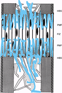
mineralize. These early bone spicules, called the primary
mineralization front (PMF), extend from each corticotomy surface toward
the central FIZ, resembling stalactites and stalagmites (3).
This osteogenic process is seen uniformly covering the entire cross
section of the cut bone, including periosteum, cortex, and medullary
spongiosa (Fig. 32.2).
 |
|
Figure 32.2.
Distraction osteogenesis, week 2. As the gap widens, the local blood supply intensifies on either side of the fibrous interzone, where microcolumns of new bone are produced by clusters of osteoblasts. These new bone cones form two primary mineralization fronts (PMF) located on both sides of the fibrous interzone. |
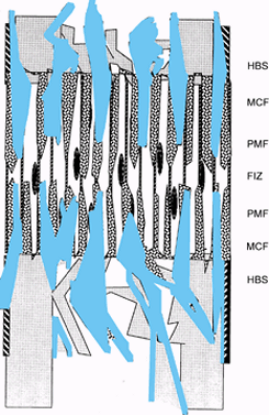
FIZ undulating across the center at an average thickness of 6 mm. As
the distraction gap increases, the bridge is formed by the elongation
of the new bone spicules. The tips of the spicules have a diameter of
about 7–10 microns, while their bases have diameters of up to 150
microns at the corticotomy surfaces. Each microcolumn of new bone is
surrounded by large, thin-walled sinusoids; this zone is called
microcolumn formation (MCF) (Fig. 32.3) (17).
 |
|
Figure 32.3.
Distraction osteogenesis, week 3. As distraction continues, length is gained by increasing the length of individual bone columns in the zones of microcolumn formation (MCF). The central fibrous interzone remains relatively avascular, while the large vascular sinuses continue to supply the areas of new bone formation at the primary mineralization fronts. |
 |
|
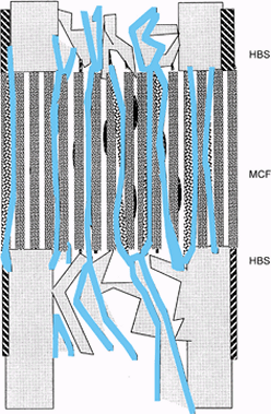
Figure 32.4.
Postdistraction consolidation. The microcolumns of bone and vascular sinuses bridge the fibrous interzone, leaving a uniform cross-sectional bridge of living bone tissue. |
The bony columns take on the staining characteristics of mature
lamellar bone, with cement lines and smaller osteocytes resting in
lacunae. The fibrovascular tissue that filled the spaces around bone
columns is replaced by normal-appearing marrow elements (1,2 and 3,6,7).
 |
|
Figure 32.5.
The microcolumns of bone are easily remodeled into the cortex and medullary canal. Neovascularity has receded and bone-marrow elements fill the intramedullary spaces. |
Each column of new bone is completely surrounded by large vascular
sinusoids. The clusters of osteoblasts that appear at the tip of each
column are in close proximity to these sinusoids. India ink injection
studies with Spalteholz clearing technique demonstrate that these
vessels parallel the bone columns and the distraction force; however,
very few vessels actually cross the FIZ, which remains relatively
avascular (1,4).
intensely hot region with a central cool area corresponding to the FIZ.
The orderly zones of bone formation seen in normal distraction
osteogenesis involve collagen deposition, osteoid formation, and
mineralization.
or bone-fixator instability, inadequate consolidation period, poor
regional or local blood supply, and a traumatic corticotomy. It is easy
to postulate that an initial diastasis would inhibit the formation of a
primary fibrovascular bridge. Instability results in macromotion,
especially shear forces that can disrupt the delicate bone and vascular
channels. The importance of rate and rhythm may well involve the
biosynthetic pathways on the cellular level by rate-limiting steps such
as protein synthesis and mitosis. Peripheral vascular disease may limit
regional vascularity, and a traumatic corticotomy can severely disturb
the local blood flow.
helpful to assess the progress of bone formation. Early on, the surgeon
can adjust the latency to enhance osteogenic potential. During
distraction, rate or rhythm adjustments may be necessary to optimize
osteogenesis. During consolidation, it is important to know when the
osteogenic area is strong enough to remove the fixator.
for completeness by intraoperative fluoroscopy, distracting no more
than 2 mm, angulating no more than 10° to 15°, and rotating no more
than 20° to 30°. Often, the far cortex is incompletely fractured or cut
through, allowing some diastasis, but multidirectional angulation will
be blocked and rotation will be eccentric. The corticotomy must be
complete to allow uniform distraction.
as the frame is fully assembled, to decrease local hemorrhage and to
ensure that the osteogenic bridge is not compromised (Fig. 32.6).
Either excess bleeding (local arterial injury) or lack of bleeding
(systemic disease or local vascular insufficiency) at the time of
corticotomy may indicate a local vascular deficiency. In these cases,
the latency can be extended by up to 14 days; premature consolidation
may occur as early as 14 days in the metaphyseal region and as early as
21 days in the diaphyseal region.
 |
|
Figure 32.6.
Low-energy corticotomy technique in the adult canine tibia. Subperiosteal placement of a narrow osteotome allows the cortex to be cracked on two sides while the periosteal tube and spongiosa are preserved. With a torquing maneuver, the third and final side can be separated. A temporary diastasis of 2 mm is acceptable to ensure complete separation of the cortices. The cortical surfaces should be reopposed with the external fixator and the periosteal tube closed. |
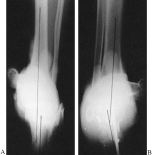
check on the progress of the distraction gap (length and alignment).
Usually, by the third week of distraction new bone mineral appears as
fuzzy, radiodense columns extending from both cut surfaces toward the
center (Fig. 32.7). Perform orthogonal views parallel to adjacent fixator rings and between connecting rods at each visit for comparison.
 |
|
Figure 32.7. A: After 7 days of distraction, the lateral view of a corticotomy shows an empty distraction gap. B:
One week later. After 14 mm of distraction, the gap is filled by radiodense new bone extending from each surface toward a central radiolucent area, the fibrous interzone. |
undulating radiolucent zone 4–8 mm wide, while more and more new bone
is added from each end. The new bone should span the entire
cross-sectional area of the host bone surfaces on both orthogonal
views. If the new bone appears to be bulging and the FIZ is narrowing,
then accelerate the distraction rate (14). If the new bone forms an hourglass appearance and the FIZ is widening, decelerate the distraction rate (9). The absence of new radiodensity
by the third week of distraction may be cause for concern (2,3,9).
Ultrasound can be used to diagnose cyst formation in the gap, which may
require bone grafting. Ischemic fibrous tissue in the gap is an
alternative explanation to delayed mineralization on the radiograph,
and this may respond to slowing the distraction rate.
monthly basis until the osteogenic area has cortex and medullary canal
on orthogonal views. Despite the appearance of these radiographic
findings, the overall bone density may be severely reduced. Any area
within the distraction gap that is less than 60% of the density of the
normal side is at increased risk to buckle under normal loads.
expert bone histologist, who has persevered with enthusiasm for many
exciting years of discovery.
scheme: *, classic article; #, review article; !, basic research
article; and +, clinical results/outcome study.
Chemistry and Biology of Mineralized Tissues. Proceedings of the Third
International Conference on the Chemistry and Biology of Mineralized
Tissues. New York: Gordon & Breach, 1988:807.
GA. The Tension-Stress Effect on the Genesis and Growth of Tissues:
Part I. The Influence of Stability of Fixation and Soft-Tissue
Preservation. Clin Orthop 1989;238:249.
GA. The Tension-Stress Effect on the Genesis and Growth of Tissues:
Part II. The Influence of the Rate and Frequency of Distraction. Clin Orthop 1989;239:263.
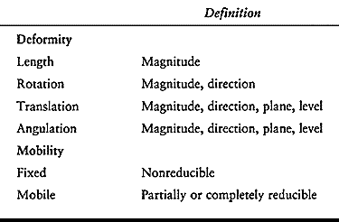
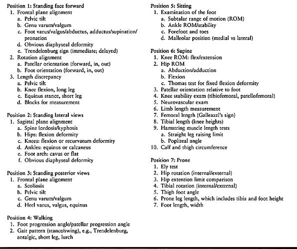
deformity may include abnormalities of length, rotation, translation,
or angulation (Table 32.1). Several other
components of limb deformity should also be considered in individual
cases: deficiency, malformation, contour, circumference, and proportion.
 |
|
Table 32.1. Limb Deformity Parameters
|
anatomy for comparison. In the lower limb, this usually is evaluated
from long anteroposterior (AP) and lateral (LAT) radiographs taken in
the standing position. The two considerations in evaluating the frontal
plane mechanical axis of the lower extremity are joint alignment and
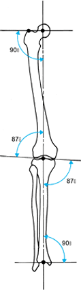
joint orientation (29). The normal alignment of
the hip, knee, and ankle joint centers is colinear. Frontal plane
deformities lead to a mechanical axis deviation, which primarily
affects the knee but also affects the subtalar, ankle, and hip joints.
Normally, the line of weight-bearing force from the ankle to the hip
joint passes through the medial tibial spine in the center of the knee (12,18). In mechanical axis deviation, it passes medial or lateral to the center of the knee.
joint to the mechanical axis line. Each joint has a normal anatomic
inclination to both the mechanical axis and the anatomic axis of the
limb segment (Fig. 32.8) (29).
In the tibia, the mechanical and anatomic axes are the same, but in the
femur they are different. The mechanical axis of the femur is defined
as the line from the center of the hip to the center of the knee. This
usually subtends a 6° angle to the anatomic axis of the femur, which
runs from the piriformis fossa to the center of the knee joint. The
knee joint line has been measured to be about 3° off the perpendicular,
so that the distal femur is in slight valgus and the tibial diaphysis
in slight varus.
 |
|
Figure 32.8.
The normal mechanical axis and joint orientation of the hip, knee, and ankle. The two components of the frontal plane mechanical axis are colinearity of the hip, knee, and ankle axis; and joint orientation of the hip, knee, and ankle relative to the mechanical axis in the angles shown. |
the femoral side as do the other two joints. The orientation of the hip
on the AP view can be characterized by the neck-shaft angle or by the
line from the tip of the greater trochanter to the center of the
femoral head. The radiographic projection of the neck-shaft angle,
which defines the relationship of the femoral head to the anatomic
axis, varies with hip rotation. The normal neck-shaft angle range is
125° to 131° (18,33).
The diameter of the femoral head is about equal to the distance from
the center of the femoral head to the tip of the trochanter. This
defines the length of the neck of the femur. A line from the tip of the
trochanter to the center of the femoral head defines the joint
orientation of the hip. Its relationship to the mechanical axis does
not change much with rotation. This relationship is 90° ± 3° (3).
preoperative planning and in determining the deformity of each bone
segment. Population norms for these lines have been
measured (3).
However, if the patient has a normal side that falls within the normal
standard deviation, then use the specific angles from that side.
orientation of the calcaneus to the tibia. The central axis of the body
of the calcaneus is normally parallel with that of the tibia in the
frontal plane. Due to the sustentaculum, the mid-body axis of the
calcaneus is laterally translated relative to the mid-tibial axis (Fig. 32.9) (29).
 |
|
Figure 32.9. Weight-bearing axis at the ankle and subtalar joints. (A) Normally, the central axis of the calcaneus is parallel and laterally displaced to that of the tibia. (B)
When there is varus or valgus deformity in the ankle or subtalar joint, the heel will be inclined into varus or valgus, relative to the tibia. The amount of the deformity can be measured directly. |
by the sourcil, which is normally horizontal to the ground with a level
pelvis (2). The center-edge (CE) angle defines the depth of the acetabulum. The normal CE angle is 20° to 30° (20).
Higher values occur in protrusio acetabulum, while lesser angles are a
feature of a dysplastic acetabulum. The pelvis is normally
perpendicular to the spine in bipedal, equal leg-length stance. The
weight-bearing axis through the pelvis to the hip joint is oriented 16°
to the vertical (21).
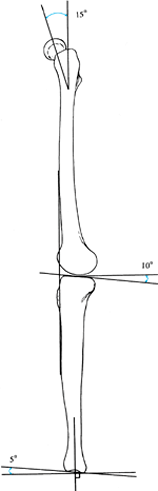
The proximal tibial articular surface has 8° to 12° of posterior tilt,
while the distal tibial articular surface has 5° of anterior tilt
relative to the mid-lateral axis (Fig. 32.10) (13).
 |
|
Figure 32.10.
The normal alignment and joint orientation on the long LAT view is marked. The mechanical axis line normally runs anterior to the midpoint of the femoral and tibial condyles. The inclination of the femoral neck varies between 5° and 15° of anteversion. The inclination of the proximal tibia varies between 8° and 12° of posterior tilt. The inclination of the distal tibia is approximately 5° of anterior tilt. |
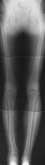
Include the hip, knee, and ankle on the same radiographic view, with
the patella pointing forward. A 3-ft radiograph is long enough for
patients under 5‘5” tall; for those over this height, a 51-in. x-ray
cassette is needed to see the alignment of all three joints on one film
(Fig. 32.11).
 |
|
Table 32.2. Clinical Evaluation Algorithms for Lower Limb Deformity
|
 |
|
Figure 32.11.
A 51-in cassette is used to assess most adults. This provides a radiograph extending from the ground to the top of the pelvis. Notice that the patella should be centered over the middle of the femur to ensure proper alignment (left knee). If the patella points inward or outward (right knee), the alignment measurements will be misleading. |
radiographic assessment of fixed pelvic obliquity and scoliosis. This
is best done by using blocks to equalize limb length and taking an
erect AP x-ray of the pelvis and spine. Hip abduction and adduction
radiographs may be necessary
to
rule out fixed pelvic obliquity on the basis of hip pathology and
limitation of motion. Knee flexion deformity alters the alignment and
length measured radiographically. Assess axial foot malalignment using
a long axial radiograph that superimposes the axial view of the os
calcis on the tibia. This can be useful to quantify the malalignment
accurately (Fig. 32.9) (29).
than frontal plane alignment, since it is in the plane of motion of all
three joints. Obtain a long LAT radiograph of the femur and tibia in
full knee extension centered over the knee (Fig. 32.10).
Normally, the anterior surface of the distal femur is colinear with the
anterior crest of the tibia in full extension. Similarly, a line drawn
from the center of the hip to the center of the ankle will pass
anterior to the midpoint of the knee on the LAT view. If lengthening is
considered, the LAT view of the knee in full extension is important for
evaluating knee subluxation, and for comparison in case of future knee
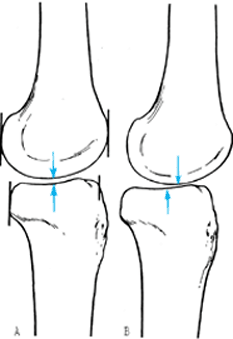
subluxation. The midpoint
of the femoral condyles on the LAT view is normally colinear with the midpoint of the tibial condyles in full extension (Fig. 32.12A). Any break in this line in full extension represents a subluxation (Fig. 32.12B) (24).
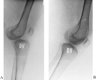
If the knee subluxes or dislocates in extension, it is important to
obtain a lateral radiograph in the degree of flexion where the knee
reduces (Fig. 32.13).
 |
|
Figure 32.12.
When there is subluxation of the knee, the radiographic changes may be subtle. Subluxation of the knee can be defined on the LAT radiograph as a step in the midpoint of the femoral and tibial condyles. Normally, these two points are opposite each other (A). When there is a subluxation of the knee, the midpoint of the tibia will displace anteriorly or posteriorly away from the midpoint of the femur with the knee in extension (B). |
 |
|
Figure 32.13. A: The knee is dislocated in full extension. B: In 30° of flexion, the knee reduces.
|
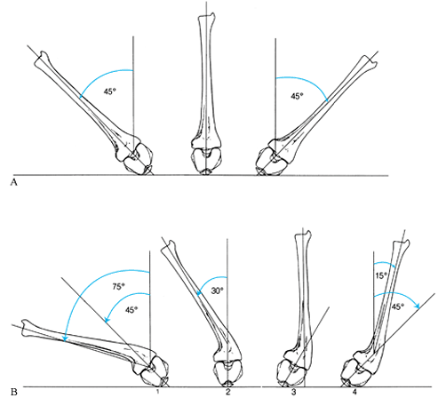
frog-leg view in adults. Anteversion of the neck can be evaluated, as
can head and neck deformities. LAT views of the ankle may be necessary
in both flexion and extension to evaluate limitation of motion and its
etiology (bone or soft tissue).
Three-dimensional reconstruction CT scans are useful for the assessment
of intraarticular deformities, especially those associated with joint
deficiencies. Three-dimensional CT scans may one day be useful for
planning deformity corrections.
 |
|
Figure 32.14. A:
Hip rotation is most accurately measured in the prone position. When the tibia is normal, the zero position is with the leg vertical. Notice that the patella points toward the examining table and the femoral condyles are horizontal. Rotation in one direction is internal; in the other direction it is external. The number of degrees is measured from the zero position. B: In the second series of diagrams, the same examination is performed for a 30° valgus deformity of the tibia. If the range of motion of the femur is judged from the tibial shaft, an incorrect assessment of 15° internal rotation (part 4) to 75° external rotation (part 1) will be made. The zero point should be selected with the patella pointing down and the femoral condyles level (part 2). The correct range of femoral rotation (45° internal to 45° external) may then be determined. |
resonance imaging (MRI) may be useful to visualize the contour of the
joint surface and assess joint laxity, contracture, and luxation.
The joint lines of the distal femur and proximal tibia will be at an
angle to each other on a standing radiograph; stress views will reveal
the full extent of the laxity. If this is not corrected together with
the deformity, then abnormal loading of the plateaus will continue
despite limb realignment.
 |
|
Figure 32.15. A: The lateral collateral ligament is lax (left).
On single-leg stance during gait, the adductor moment arm leads to a varus deformity through the knee joint. The lateral joint line opens to the point that the lateral collateral ligament becomes tight (center). With descent of the fibular head, the lateral collateral ligament can be tightened to correct the articular varus deformity (right). B: The medial collateral ligament is lax (left). Associated with a valgus deformity, the tibia subluxes laterally (middle). The medial collateral ligament can be retensioned by distraction of an osteotomy located proximal to its insertion (right). The distal end of the osteotomy runs distal to the tibial tubercle to avoid pulling the patellar tendon down. |
asymptomatic. Deformity symptoms include pain and inflammation around
joints, apparent or real joint restriction of motion, and gait
dysfunction or alteration. Patients also present with aesthetic and
psychosocial complaints regarding limb deformities.
relieve symptoms if present and to protect adjacent joints from
development of osteoarthrosis secondary to the deformity. Without good
data about the natural history of asymptomatic deformities and their
contribution to later joint degeneration, it is difficult to specify
exact indications for their surgical treatment (8,9,11,16,18,21,26,30,31 and 32).
Isolated rotational deformities should not be treated unless
symptomatic. They should be corrected as part of a comprehensive
approach to the treatment of lower limb alignment.
treatment, even in asymptomatic patients: distal femoral mechanical
valgus greater than 5°, proximal tibial mechanical varus greater than
5°, and mechanical axis deviation greater than 15 mm. Other
asymptomatic deformities should be considered for correction
prophylactically if radiographic evidence of degenerative joint disease
is seen or if only clinical signs are detected (e.g., a positive
Trendelenburg sign in a dysplastic hip, lateral thrust in a varus
knee). Other deformities that should be considered for treatment
include procurvatum deformity of the distal tibia greater than 15°,
recurvatum deformity of the distal tibia greater than 10°, and varus or
valgus deformity of the distal tibia greater than 10° when subtalar
joint motion is restricted. Although these guidelines for deformity
correction are based on the available literature, each patient must be
evaluated individually.
deformity and not create a deformity in an effort to treat one. The
best example is distal femoral valgus. Recommended treatment for genu
valgum has included distal femoral osteotomy or proximal tibial
osteotomy (Fig. 32.16) (7,9,28).
An isolated deformity in the femur should never be treated by a
corrective osteotomy of a normal tibia. This will lead to persistent
joint inclination and eventual subluxation. Cooke et al. demonstrated
that for combined distal femoral and proximal tibial deformities, the
best operation is a corrective osteotomy at both levels (4,5).
The first step in deformity correction, therefore, is to assess the deformity by accurately defining and describing it (Table 32.1, Table 32.2); then preoperative planning begins.
 |
|
Figure 32.16.
A high tibial osteotomy was performed to correct a valgus deformity of the distal femur. In addition to the sloped joint orientation that was present preoperatively, the patient is now developing collapse into varus and lateral subluxation. This illustrates why a normal tibia should not be osteotomized to correct for a deformity in the distal femur. |
while the apices of metaphyseal and especially of juxtaarticular
deformities are subtle or less clear. The first step is to determine
the level of the apex of the angular deformity. With diaphyseal
deformities, draw a line down the concave or convex cortex proximal and
distal to the apex. The intersection of these two cortical lines is the
true apex of deformity. For juxtaarticular and metaphyseal deformities,
a more complex system is necessary to determine accurately the level of
the deformity’s apex.
Required materials are a standing radiograph with the patella pointing
forward, knee in extension, from hips to ankles, of both lower limbs,
and a pencil, a long straight edge, and a goniometer or protractor.
 |
|
Figure 32.17. The malalignment test. This test determines the origin of frontal plane malalignment. Step 0:
Draw HA, the mechanical axis line of the lower limb, from the center of the femoral head to the center of the ankle plafond. If this line passes medial to the medial tibial spine, there is medial mechanical axis deviation (MAD). If it passes lateral to the center of the knee, there is lateral MAD. Step 1: Draw HK, the mechanical axis of the femur, from the center of the femoral head to the center of the knee. Draw FC, the femoral condyle line. Measure the lateral angle HKF. This should be 87° ± 2°. Outside these limits, the femur is contributing to the MAD. Step 2: Draw KA, the tibial mechanical axis line, from the center of the knee to the center of the ankle. Draw the tibial plateau line TP. Measure the medial angle AKP. This should be 87° ± 2°. Outside these limits, the tibia is contributing to the MAD. Step 3: Compare the orientation of FC to TP. These should be parallel to each other. If they diverge more than 1° to 2°, there is joint laxity contributing to MAD. A: Femoral malalignment. B: Tibial malalignment. C: Joint laxity malalignment. |
then steps 1 to 3 will indicate whether the deviation is in the femur
or the tibia. If lines FC and TP are not parallel, then there is an
intraarticular component to the mechanical axis deviation.
apex of an angular deformity. The choice of level is influenced by the
proximity to the adjacent joint, the type of fixation, skin coverage,
bone quality, and, in children, the physis. A deformity apex within the
bone’s metaphysis or diaphysis is suitable for osteotomy and fixation.
A juxtaarticular deformity apex presents difficulties with both the
osteotomy and fixation. In children, correcting a juxtaarticular
deformity would cause a transphyseal separation, whereas in adults such
a correction would necessitate a periarticular or intraarticular
osteotomy. Therefore, the practical level for osteotomy is usually
within the metaphysis in these deformities. For this reason, the
metaphyseal and diaphyseal deformities will be grouped together under
the name metadiaphyseal; the juxtaarticular type of deformity will be considered separately.
the malalignment test, ascertain the apex of deformity. The osteotomy
level can then be determined, taking into consideration the limitations
imposed by the joint and physis and by the fixation method.
Preoperative determination of tibial deformity with a normal femur is
shown in Fig. 32.18 and Fig. 32.19.
 |
|
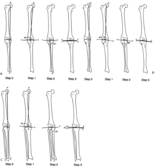
Figure 32.18. A:
The apparatus for correction of this angular deformity is preconstructed with two levels of fixation on either side of the hinge. The hinge level, plane, magnitude, and direction are built into the apparatus. Tibial diaphyseal deformity with a normal femur. Step 0: Draw the mechanical axis line to demonstrate the degree of mechanical axis deviation created by the obvious tibial diaphyseal deformity. The malalignment test was performed to confirm that the orientation of the distal femur is normal. Step 1: Since the femur is normal, draw the line from the center of the hip through the center of the knee and extend it distally. This is the mechanical axis of the proximal tibia. Step 2A: Draw a line from the center of the plafond extending proximally in line with the anatomic axis of the tibia. This is the mechanical axis of the distal tibia. The center of rotation of angulation is at the intersection of the two mechanical axis lines. The angular deformity measures 26°. Step 2B: The alternative method is to draw a line down the convex cortices of the deformity. These lines intersect at the same level and also demonstrate a 26° deformity. Step 3A: The deformity correction is performed on paper at the level of the apex of the deformity for a total of 26°. This realigns and overlaps the mechanical axis lines to reestablish the colinearity of the hip-knee-ankle axis. Step 3B: After opening wedge correction. This osteotomy also realigns the diaphyseal line of the convex cortex so that it is colinear. B: Tibial frame applied to correct deformity illustrated in A. |
 |
|
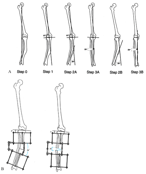
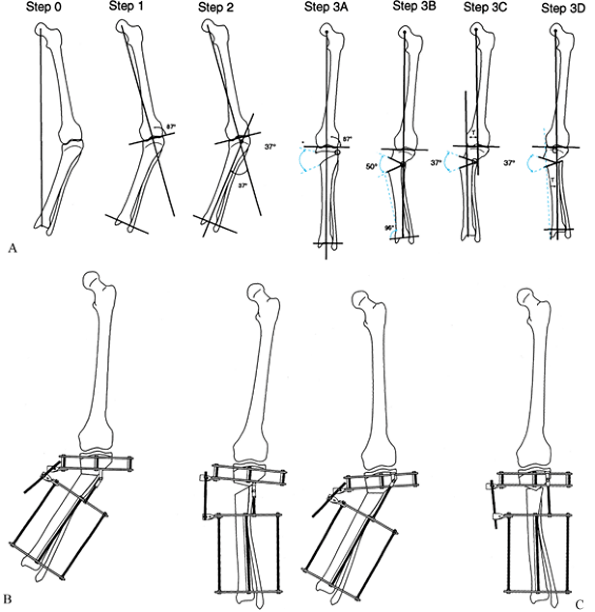
Figure 32.19. A: Juxtaarticular tibial deformity with a normal femur. Step 0:
Draw the mechanical axis line from the center of the femoral head to the center of the ankle. The malalignment test was performed to confirm that the varus mechanical axis deviation is due only to the tibia and that the femur is normal. Step 1: Draw the mechanical axis line of the femur and extend it distally. This is the mechanical axis of the proximal tibia. Step 2: Draw the line from the center of the ankle plafond extending proximally parallel to the anatomic axis of the tibia. This is the mechanical axis of the distal tibia. Note that the level of intersection of the two mechanical axis lines is at the level of the growth plate. The angular deformity measures 37°. Step 3A: The deformity may be corrected by a 37° opening wedge through the growth plate, thus realigning the mechanical axis and reestablishing normal joint orientation. Step 3B: Correction of the deformity at the level of the tibial metaphysis requires a 50° correction to realign the mechanical axis. This creates a malorientation of the knee and ankle. Notice that the mechanical axis now subtends a 96° orientation to the ankle joint instead of the normal 90°. Step 3C: If only 37° of deformity is corrected, then there is persistent varus mechanical axis deviation. The knee and ankle are oriented correctly to each other, but the mechanical axis is deviated due to a persistent translational deformity (T). Step 3D: To realign the mechanical axis at the level of the metaphysis, which is distal to the apex of the deformity, the correction should include both 37° of angular correction and lateral translation in the amount of T. The magnitude of T increases as the level of the osteotomy moves farther away from the apex of the deformity. B: If the hinge is placed at the level of the osteotomy, overcorrection is required to eliminate mechanical axis deviation. Note that the rings are not parallel at the end of correction because of overcorrection. C: The apparatus is preconstructed with the hinge at the level of the center of rotation of angulation. This leads to angulation and translation. The rings are parallel at the end of correction. |
When the apex of the deformity is metadiaphyseal, do the osteotomy at
the level of the apex, and place the hinge at the level of the apex.
The correction angulates the bone ends. When the apex of the deformity
is juxtaarticular, perform the osteotomy in the metaphysis at a level
different from that of the apex, and place the hinge at the level
of the apex. The correction causes translation and angulation of the bone ends.
 |
|
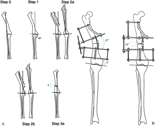
Figure 32.20. A: Diaphyseal femoral deformity with a normal tibia. Step 0:
Draw the line from the center of the femoral head to the center of the ankle, demonstrating a valgus mechanical axis displacement. The malalignment test confirms a normal tibial alignment. Step 1: Draw the mechanical axis line of the tibia from the center of the ankle to the center of the knee and extend it proximally. This is the mechanical axis of the distal femur. Step 2a: Draw the mechanical axis line of the femur on the opposite normal side. Draw the anatomic axis line of the normal side down the midshaft of the proximal femur. Measure the angle between the mechanical and anatomic axes (α). Draw the anatomic axis of the proximal femur on the deformed side. Draw a line from the center of the hip parallel to the anatomic axis. Step 2b: Draw a line from the center of the hip extending distally at α degrees to the last line. This is the mechanical axis of the proximal femur. This line intersects the distal mechanical axis line at the apex of the deformity, demonstrating a 15° angular deformation. Step 3a: Correct the angular deformity through an osteotomy at the level of the apex of the deformity. The angular correction required to realign the mechanical axis is 15°. B: Apparatus before and after open-wedge correction with hinge at osteotomy level. |
 |
|
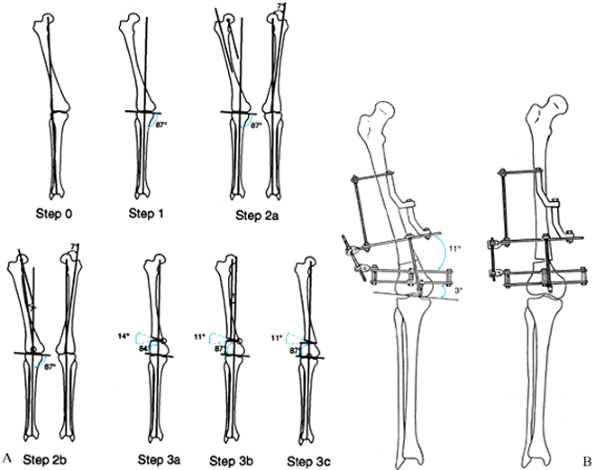
Figure 32.21. A: Juxtaarticular femoral deformity with a normal tibia. Step 0:
Draw the mechanical axis line from the center of the hip to the center of the ankle. This line passes lateral to the center of the knee, indicating a valgus mechanical axis deviation. The malalignment test confirms that the tibial alignment is normal. Step 1: Draw the mechanical axis line from the center of the ankle through the center of the knee and extend it proximally. This is the mechanical axis of the distal femur. Step 2a: Draw the mechanical axis line of the femur on the opposite normal side. Draw the anatomic axis line of the normal side down the midshaft of the proximal femur. Measure the angle between the mechanical and anatomic axes (7° in illustration). Draw the anatomic axis of the proximal femur on the deformed side. Draw a line from the center of the hip parallel to the anatomic axis. Step 2b: Draw a line from the center of the hip extending distally at 7° to the last line. This is the mechanical axis of the proximal femur. This line intersects the distal mechanical axis line at the knee joint, indicating a juxta-articular deformity measuring 11°. Step 3a: Since it is not possible to do an osteotomy so distal, the osteotomy is performed at the level of the distal metaphysis. Correction of the mechanical axis alignment by a pure angular correction at this level requires 14°, since the osteotomy is not at the level of the apex of the deformity. As in the tibial example, this produces a slight malorientation of the hip to knee joint lines. Step 3b: The correction of only 11° results in persistent valgus mechanical axis deviation. The deformity that remains is purely a translational one of amount T. Step 3c: The most accurate correction through a metaphyseal osteotomy is to combine 11° of angulation with lateral translation of amount T. T increases as the distance of the osteotomy to the true apex of the deformity increases. B: Apparatus with hinge at juxtaarticular center of rotation. Angulation and translation correction occur since the hinge is at a different level from the osteotomy. |
 |
|
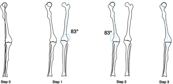
Figure 32.22. Anatomic axis method of preoperative planning for femur. Step 0:
There is a mechanical axis deviation (MAD) caused by a femoral deformity. Since there is a cup arthroplasty, the center of the femoral head, which is essential for mechanical axis planning, cannot be used. Therefore, anatomic planning is used. Step 1: Draw the anatomic axis line on the normal side down the midfemur and measure the lateral angle it subtends to the knee (83°). Step 2: Draw an 83° line from the center of the knee on the deformed side. This is the anatomic axis of the distal femur. Step 3: Draw the anatomic axis line of the proximal femur on the deformed side (midline proximal femur shaft). The intersection point of the two anatomic axis lines is the center of rotation of the angulation. |
 |
|
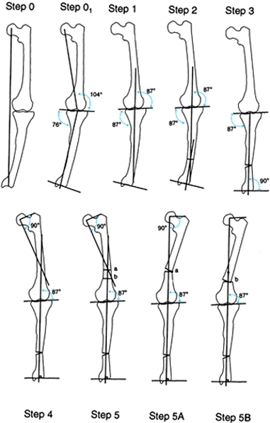
Figure 32.23. Combined femoral and tibial deformities in the absence of a normal opposite side. Step 0:
Draw the mechanical axis line from the center of the hip to the center of the ankle. This line passes medial to the center of the knee, indicating a varus malalignment. Step 01: The malalignment test demonstrates a deformity in both tibia and femur. Step 1: Draw a line 87° to the knee orientation line. Extend this line both proximally and distally. Step 2: Draw a line perpendicular to the ankle plafond (or distal tibial shaft) and extend this line proximally. Step 3: Correct the tibial deformity at the level of the apex of the deformity, realigning the tibial mechanical axis and reorienting the ankle and knee. Extend the normalized tibial mechanical axis proximally. Step 4: Draw the mechanical axis of the proximal femur. If there is a normal opposite femur to compare, use the angle measured from the opposite side. If there is not a normal angle, use 90°. The intersection point indicates the apex of the deformity. Step 5: The osteotomy can be performed at the level of the intersection of the axes (a) or at a lower level (b). Step 5A: Draw the osteotomy at the level of the apex of the deformity, realigning the femoral mechanical axis with that of the tibia. Since this deformity is a bowing of the femur and not truly a uniapical angular deformity, the correction produces a sharp angulation in the cortex of the femur which may be associated with a cosmetic deformity. Step 5B: The osteotomy may be performed at a lower level combined with translation, to minimize the angulation in the shaft of the femur. This produces a better aesthetic appearance. The center of rotation of the second osteotomy (b) is still at level a. |
the level of the osteotomy. The apex may not always be the optimal
level or even a possible place to perform the osteotomy for several
reasons. In developmental and congenital deformities, the deformity is
often at the level of the growth plate or joint and, therefore, is
inaccessible for fixation or osteotomy. Angular corrections performed
as opening or closing wedges not at the level of the apex of the
deformity create secondary translational deformities (Fig. 32.24).
To avoid this, the bone ends must be translated either acutely or by
using a translation hinge. The translation needed can be minimized by
performing the osteotomy as close as technically feasible to the true
apex of the deformity. An alternative technique uses a hinge at the
level of the osteotomy, correcting angulation first, followed by
translation by modifying the frame.
 |
|
Figure 32.24. Secondary translational deformities. A:
The so-called golf club deformity of the distal femur is a result of repeated closing wedge varus osteotomies in the supracondylar metaphyseal region of the femur for the treatment of a juxtaarticular deformity of the distal femur. This produces a progressive medial translational deformity with each successive osteotomy. B: Medial translational deformities of the tibia are the result of repeated valgus osteotomies at the metaphyseal diaphyseal junction for the treatment of these juxtaarticular deformities of the tibia. In the right tibia, overcorrection was carried out to realign the mechanical axis similar to that described in Fig. 32.19, step 3B. On the left, the ankle and knee joints were reoriented but the mechanical axis was not fully corrected, leading to a persistent varus from the translational component of the deformity. C: A varus deformity of the distal tibia due to a malunion was treated by a supramalleolar osteotomy to realign the ankle to the knee joint. This correction ignores the mechanical axis deviation created by the malunion. It demonstrates again that angular correction not at the level of the apex of an angular deformity leads to a translational deformity. |
contraindicated at the apex include the presence of soft-tissue
coverage problems or avascular, sclerotic, or previously infected bone
(suboptimal for osteotomy). A translational correction of the osteotomy
at a level above or below the apex is required.
level is in the proximal or distal metaphysis. It may be preferable to
perform a metaphyseal-level corticotomy followed by a translational
correction to realign the mechanical axis for both angulation and
translation, or to perform two osteotomies, one for lengthening and one
for deformity correction.
translational deformities. The translational component may either
compensate or aggravate the mechanical axis deviation produced by the
angular deformity. In the tibia, if translation is in the direction
opposite the angular deformity, then the translation will produce a
compensatory effect on the mechanical axis deviation. While this
translation may not completely realign the mechanical axis, it will
reduce the amount of deviation (Fig. 32.25). On the other hand, if the translation is in the same direction
as the angular deformity, the mechanical axis deviation will be
aggravated. The apex of the deformity in these cases is not at the
malunited level of the two bone segments. Because of the translation,
the true apex of the deformity will be either proximal or distal,
depending on whether the translation is aggravating or compensatory. In
the tibia, compensatory deformities will have an apex distal to the
level of the malunion, but aggravating translational angulation
deformities will have a true apex proximal to the level of the malunion.
 |
|
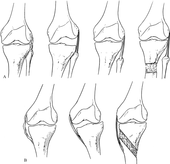
Figure 32.25.
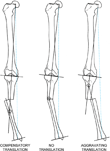
Angular malunions of the tibia lead to varying degrees of mechanical axis deviation, depending on the degree of angulation, the level of the malunion, and the magnitude and direction of any associated translational deformity. These three varus malunions differ only in the magnitude and direction of the translational component of the malunion. The center malunion has pure angulation without translation of the bone ends. The malunion on the left has the same degree of angulation combined with translation toward the convexity of the deformity. The malunion on the right has the same degree of angulation combined with translation toward the concavity of the deformity. Notice the amount of mechanical axis deviation (MAD) in all three examples. The MAD is decreased when the translation is toward the convexity and increased when it is toward the concavity. The former is called compensatory translation, whereas the latter is called aggravating translation. Notice the point of intersection of the mechanical axis lines of the proximal and distal tibia. When there is no translation, the intersection is at the level of the malunion. When there is a compensatory translation, the intersection point is distal to the malunion. When there is aggravating translation, the intersection point is proximal to the malunion. The intersection point is considered to be the true apex of the angulation-translation deformity, while the malunion is considered to be the apparent apex. |
By performing the osteotomy at the level of the true apex—the
intersection point of the mechanical axis—the limb will realign both
angulation and translation through a single hinge (Fig. 32.27). A translating hinge apex offers the added advantage of allowing an osteotomy
through healthy bone rather than through a sclerotic, avascular, previously open, or infected region at the deformity’s apex.
 |
|
Figure 32.26.
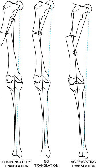
Varus malunions of the femur are illustrated with and without aggravating or compensatory translation. Notice that in the femur, translation toward the convexity is aggravating, whereas translation toward the concavity is compensatory. The reason for this is that by convention we refer to translation as the distal fragment being translated relative to the proximal. If we think of the proximal fragment of the femur as the one that is translating, then the rules are similar to that described in the tibia (Fig. 32.25). Notice that the translational deformity shifts the true apex of the deformity either proximal or distal to the apparent apex at the level of the malunion. |
 |
|
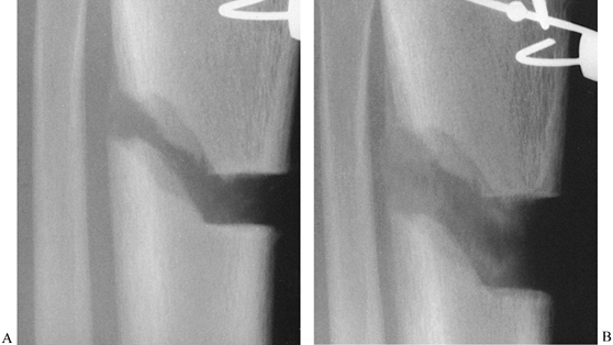
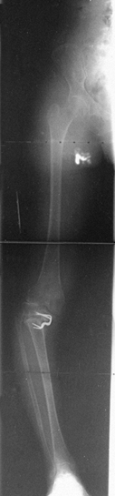
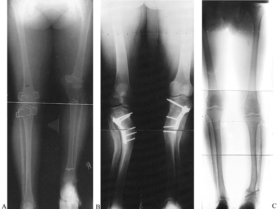
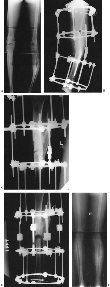
Figure 32.27. A: Varus malunion of the mid diaphysis of the tibia with compensatory lateral translation. B:
The frame was applied with the hinges at the level of the true apex of the deformity, and the corticotomy was carried out at that level. C: Distraction of the concavity led to realignment of the tibia through an open-wedge correction. Notice the simultaneous correction of the angulation and translation, as demonstrated by the colinearity of the medial tibial diaphysis. The hinges are now straight and the rings are parallel, indicating completion of the deformity correction. D: After completion of the angular correction, the parallel rings were distracted to lengthen the tibia. E: Final AP standing radiograph demonstrates the alignment of the corrected malunion. There is a persistent leg-length discrepancy of 2 cm, which was accepted because of slow healing in this patient. |
osteotomy at the level of the true apex. An osteotomy at the true apex
corrects both angulation and translation of the malalignment
simultaneously, but it does not correct any contour deformity created
by the translated bone ends (Fig. 32.28). If
the contour deformity is significant, then the osteotomy should be done
at the level of the malunion. Translation and angulation must be
corrected separately.
 |
|
Figure 32.28. A:
Valgus malunion of the mid diaphysis of the tibia with aggravating lateral translation. There was a significant contour deformity created by the malunion. Preoperative planning demonstrates that the true apex of the deformity is proximal to the level of the malunion. Angular correction at this level simultaneously corrects for the translational component of the deformity. B: This leaves a persistent contour deformity that was unacceptable to the patient. C: Therefore, the alternative is to perform the correction at the level of the malunion to correct separately the angulation, translation, and the contour deformities. The radiograph demonstrates the angular and translational corrections, which were performed acutely followed by distraction to lengthen the tibia. D: The final radiograph demonstrates elimination of the angulation-translation and, as a result, of the contour deformity. The acute translational maneuver should be avoided because it contributes to delayed consolidation by disrupting the periosteum. It is preferable to correct the angulation gradually, followed by distraction to lengthen the tibia, followed by gradual translation. |
as varus, valgus, procurvatum, and recurvatum of the distal segment
relative to the proximal segment. The terms varus and valgus describe angular deformities in the frontal plane; procurvatum and recurvatum
describe angular deformities in the sagittal plane. Using this
convention, a deformity with varus and recurvatum is described as a
biplanar deformity. Careful analysis of most biplanar deformities
reveals that they have but a single apex; moreover, the deformity lies
in an oblique plane, somewhere between the frontal and sagittal planes (Fig. 32.29) (25,27).
We perceive the deformity as biplanar because the standard radiographic
views are obtained in the anatomic reference planes, which may be
different from the plane of angulation. Geometrically speaking,
however, two lines can subtend only one plane. If we consider each bone
segment as a line, these two lines can form an angle with each other
only in one plane, regardless of the presence of angulation, rotation,
translation, or length of deformities.
A
second plane of angulation can exist only if a second angular deformity
at another level is introduced into these bone segments or lines.
 |
|
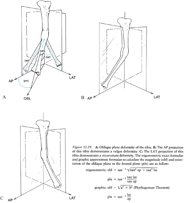
Figure 32.29. A: Oblique plane deformity of the tibia. B: The AP projection of this tibia demonstrates a valgus deformity. C:
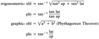
The LAT projection of this tibia demonstrates a recurvatum deformity. The trigonometric exact formulae and graphic approximate formulae to calculate the magnitude (obl) and orientation of the oblique plane to the frontal plane (pln) are as follow:Symbol |
 |
|
Symbol. No caption available.
|
true plane of a deformity in a plane oblique to the frontal plane. The
simplest method is to rotate the limb until it appears straight (Fig. 32.30) (27).
The true plane of deformity is the plane where the projection of a
deformed limb appears straight. The plane 90° to this projection should
demonstrate the maximum angulation profile of the deformity.
Radiographs taken in these two planes can be used to determine the
orientation of this plane and the magnitude of the true deformity.
 |
|
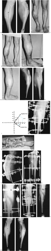
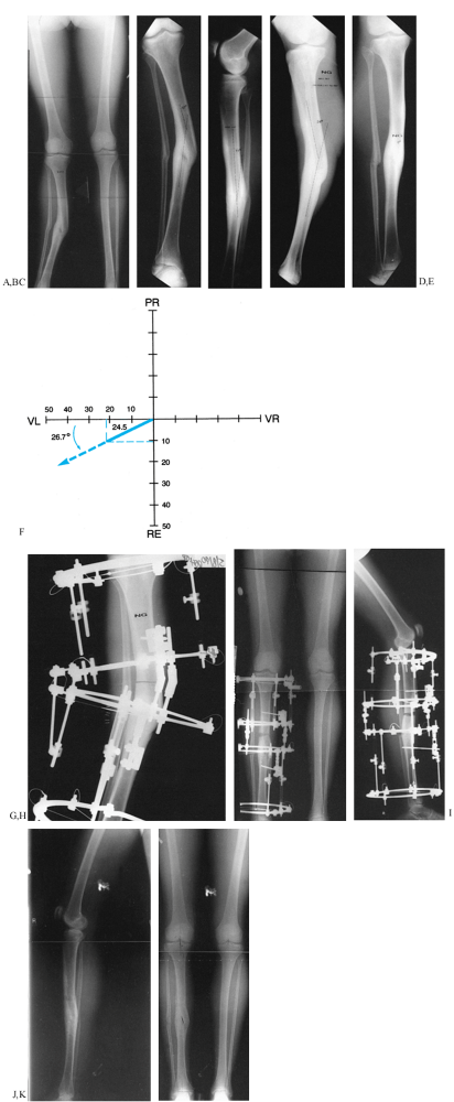
Figure 32.30. A: Malunion of the tibia with 20° of varus and 13 mm lateral translation. B: The LAT projection demonstrates 25° of procurvatum and 10 mm of posterior translation. C: Observation of the patient from the front demonstrates the varus deformity of the tibia. D: When the patient turns his foot inward, the varus deformity seems to disappear and the tibia appears straight. E: Examination from the side demonstrates the procurvatum deformity of the tibia. F: When the patient turns his foot inward again, the maximum angular profile of the deformity is seen. G: The maximum angular profile is captured radiographically on this LAT oblique view of the tibia. It measures 32°. H:
An internal rotation AP oblique radiograph. In the plane of the deformity, the tibia appears straight. The translational component of the deformity can be appreciated on this view. I: The measurement of 20° varus and 25° procurvatum were plotted on a graph. The vector obtained by the point 20–25 represents the magnitude 32° and true orientation 51.5° to frontal plane of the oblique plane angular deformity. Superimposed on this graph, the magnitudes of translation on the AP and LAT are plotted. The magnitude of the oblique plane translation is 16 mm oriented 35° to the frontal plane. The translation and angulation planes are 88° apart. This confirms the radiographic findings. J: The malunion was split obliquely. K: Notice the appearance of the apparatus in relationship to the left hinge. The hinges have been placed relative to the apex of the oblique plane deformity. Notice that the distance of the hinge rods to the central bolts differs for the medial and the lateral hinge, demonstrating that the hinges are oriented obliquely to the anatomic planes. L: A true LAT view of the deformity aligns the hinges with the apex in the oblique plane. M: In this manner, distraction of the concavity leads to realignment of the diaphysis on the LAT view of the tibia simultaneous with realignment on the AP view. N: All that remains is to correct the translational deformity. O: By applying translational rods, the tibia was narrowed, bringing the cortical ends together side to side. P: Appearance of the callus at the time of the removal of the apparatus 23 weeks after application. Notice that there is no corticalization of the callus between the bone ends. The patient was, therefore, protected in a patellar tendon bearing cast. The final AP (Q) and LAT (R) radiographs demonstrate the recurrence of deformity that occurred because of the premature removal of the apparatus prior to complete corticalization of the distraction callus. Notice also the ring sequestrum from one of the pin sites (arrow). |
The graphic method requires only a pencil and goniometer to calculate
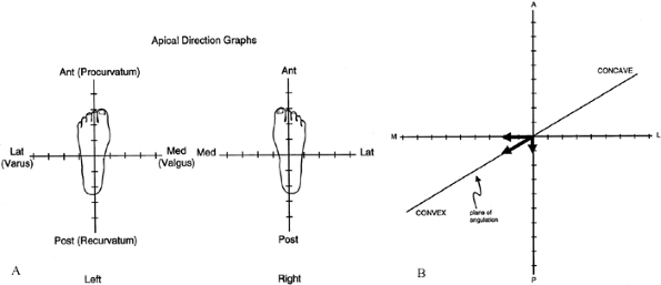
the magnitude and direction of the oblique plane deformity (Fig. 32.31). Bar and Breitfuss have published a nomogram to determine the true angular deformity and its oblique plane (1). Ilizarov plots the apical deviation from the axial midline on the AP and LAT views as x and y coordinates and determines the plane of deformity graphically (Fig. 32.32).
The Ilizarov apparatus allows the surgeon to make use of these
calculations. By determining the true plane of deformity, the surgeon
can also determine the axis of the deformity’s apex. The axis of the
deformity is always perpendicular to the plane of the deformity (Fig. 32.33).
By applying a hinge at the true apex of an oblique plane deformity
perpendicular to the true plane of this deformity, the surgeon can
simultaneously correct the AP and LAT projections of the deformity (Fig. 32.34).
Alternatively, the apparatus could be applied to correct the deformity
in the AP plane; afterward, the hinges would be reoriented to correct
the deformity in the LAT plane. This is a more time-consuming and
less-efficient method, but it is accurate.
 |
|
Figure 32.31. A: Mark the direction of the apex of angulation on the axes of the graph (as if looking down at your own feet). B: Mark the magnitude of the AP and LAT angles (1 mm = 1°; AP, x axis; LAT, y axis). The resultant vector represents plane, magnitude, and apical direction.
|
 |
|
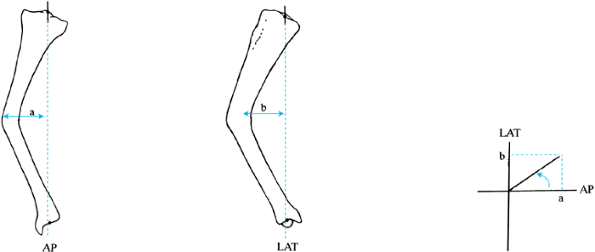
Figure 32.32.
Ilizarov’s method for determining the plane of the oblique deformity. A line is drawn from the center of the knee to the center of the ankle on both the AP and LAT views. The distance from this line to the apex of the deformity is measured on both views. These are plotted on a graph, and the orientation of the resultant vector from the AP or LAT plane is measured. This represents the plane of the apex of the deformity. |
 |
|
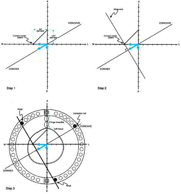
Figure 32.33. Graphic preoperative planning of hinge placement in oblique plane deformities. Step 1:
Measure the diameter of the tibia on the AP and LAT views and mark on the graph as shown. The lateral aspect of the tibia should be marked on the upper side of the y axis, and the width on the AP should be marked on the minus and plus sides of the x axis, for right and left legs respectively. These markings should be to normal scale, with 1 mm on the radiograph equal to 1 mm on the graph. The points on the x and y axes are connected with a line to form a triangle. This represents the cross section of the tibia at the level of the apex of angulation. If a different level or bone is chosen, the representative x section for that apical level should similarly be centered. Step 2: The hinge axis is always perpendicular to the plane of angulation. If an opening wedge hinge placement is chosen, it should be placed at the convex edge of the bone. The direction of the convexity is shown by the arrow. The hinge axis is therefore drawn perpendicular to the plane of the angulation axis passing tangential to the convex cortex of the bone. Step 3: To determine the hinge holes, a ring of the appropriate size for the limb should be placed on the graph. To center the ring, the reference marks of the ring must be defined. The line connecting the central bolts represents the AP axis of the frame. Since the rings are normally centered over the lateral edge of the central bolts of the ring, it should be placed on the y axis. The ring is normally spaced two fingerbreadths from the anterior skin of the leg. This can be marked on the graph by noting the thickness of the anterior skin followed by a two-fingerbreadth space anterior to that. The position of the ring on the y axis fixes it in place. The hinges are placed in the holes where the hinge line intersects the ring. The distraction rod on the concavity is placed where the plane axis line intersects the ring on the concave side of the angulation. |
 |
|
Figure 32.34. A: Valgus malunion of the tibia with aggravating lateral translation. B: The deformity measures 22° of valgus with an apex proximal to the level of the malunion. C:
On the LAT view, there is an 11° deformity, indicating that this is an oblique planar deformity with angulation and translation. D: The maximum profile of deformity is demonstrated on this oblique LAT radiograph and measures 24°. E: The radiograph in the plane of the deformity illustrates the translational component in the absence of angulation. F: Graphic determination of the magnitude and plane of the oblique deformity on a left leg graph demonstrates a 24.5° deformity oriented 26.7° from the frontal plane. (This is the same example shown in Fig. 32.29, Fig. 32.30, and Fig. 32.33.) G: The apparatus is applied so that the hinges are at the level of the true apex of the deformity which is proximal to the malunion. The corticotomy is performed at the same level. H: An open-wedge correction was carried out, realigning the mechanical axis of the lower limb. Note that all of the rings are parallel and the hinges are straight. I: On the LAT view, one can also appreciate the open wedge anteriorly with the correction of the recurvatum deformity. The rings are parallel on the lateral at the end of the correction. The follow-up AP (J) and LAT (K) radiographs demonstrate the restoration of AP and lateral alignment of the tibia. |
Since translation is a direct linear measurement and not an angular
deviation, the Pythagorean or graphic methods described are both
accurate for the assessment of translation deformities in planes
oblique to the frontal projection. Both the magnitude and the true
plane of translation can be determined.
 |
|
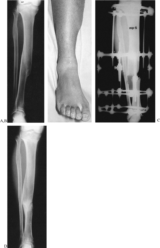
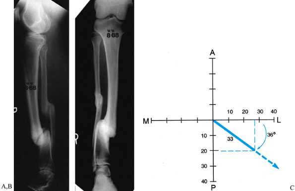
Figure 32.35. A,B:
Translational deformity may also be seen in two planes. This tibial nonunion has a posterior and lateral translational deformity. C: The posterior translation measures 2 cm, while the lateral translation measures 2.7 cm. When these are plotted on a graph, it demonstrates that the true translation is 33 mm in a plane oriented 36° to the frontal plane. This graph is drawn as for a right leg. |
plane of angulation may be the same as or different from the plane of
translation. If angulation and translation are in the same plane, they
can be characterized as a single apex of angulation (Fig. 32.36).
If this is in one of the anatomic planes (frontal or sagittal), one
view will show angulation and translation while the other shows no
deformity. If both are in the same oblique plane, the center of
rotation will be at the same level on both AP and LAT radiographs. If
angulation and translation are in different planes 90° apart, there
will be one plane with only angulation and one with only translation (Fig. 32.37).
This is readily appreciated when the deformations correspond to the
anatomic planes; translation only is seen on one view and angulation
only on the other view. If they are in different oblique planes, then
both angulation and translation are present in both AP and LAT views.
To differentiate this from angulation/translation in the same oblique
plane, one must examine the levels of the center of rotation of the
angulation on AP and LAT views. When they are in different planes, then
the center of rotation on the AP view is at a level different from that
on LAT view, usually one apex above and one below the fracture level.
Angulation and translation may also be in different planes that are
less than 90° apart (Fig. 32.37).
The graphic method of oblique plane deformity assessment can be used to
plot the plane of angulation and the plane of translation on the same
graph (Fig. 32.30). The difference in planes between angulation and translation can then be measured from the graph.
 |
|
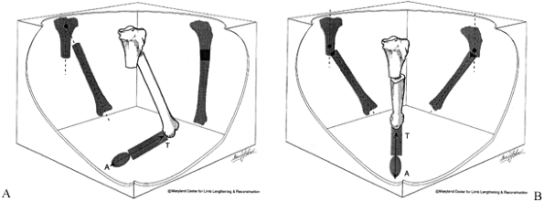
Figure 32.36. Angulation-translation deformity in the same plane. A:
Frontal plane angulation and translation. Angulation and translation are both in the frontal plane. No deformity is seen in the sagittal plane. Note that the center of rotation of the angulation is proximal to the fracture level. B: Oblique plane angulation and translation: same plane. Angulation and translation are seen on both AP and LAT views. The center of rotation of the angulation is the same on both views. This indicates that both angulation and translation are in the same oblique plane (see axial). The apical direction of angulation is marked with an arrow A and the direction of translation is marked T. This represents the same deformity shown in (A), rotated into an oblique plane. |
 |
|
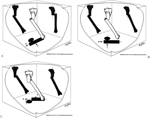
Figure 32.37. Angulation-translation deformity in different planes. A:
Frontal plane angulation with sagittal plane translation. The AP shows angulation with translation, whereas the LAT shows translation without angulation. The axial view shows the direction of the apex of angulation A relative to translation T. In this example, they are 90° apart. B: Oblique plane angulation-translation: different planes 90° apart. Angulation and translation are seen on both AP and LAT views. Note that the center of rotation is at a level on the AP that is different from that on the LAT. On the AP it is proximal to the osteotomy while on the LAT it is distal. This is the tipoff that the two are in different planes. On the axial view, the direction of angulation A and of translation T are 90° apart. This represents the same deformity shown in (A) rotated into an oblique plane. C: Oblique plane angulation-translation: different planes less than 90° apart. The AP and LAT projections are as before with angulation and translation seen on both views. The difference is that the plane of angulation A and translation T are different but less than 90° apart. This is one of the most common clinical situations. |
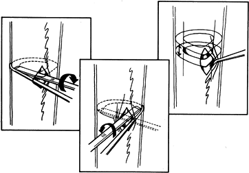
translation has ramifications on treatment. When both are in the same
plane, there is a single center of rotation point that will correct
both deformities by angulation alone. In nonunions, the hinge can be
placed at this angulation-translation point; after distracting the ends
apart, the angulation and translation are corrected by angulation
around this hinge. If there is a malunion, an osteotomy may be
performed at this level with opening or closing wedge correction. This
corrects both angulation and translation together (Fig. 32.27).
then several strategies may be pursued. Angulation may be corrected at
the apical level on the AP, LAT, or oblique views (Fig. 32.30).
Translation, if significant, will not correct with the angulation and
requires a separate correction in the LAT, AP, or oblique plane (Fig. 32.30).
Alternatively, a double-level osteotomy can be performed, correcting
angulation and translation in the frontal plane with one osteotomy at
the AP angulation-translation point and one osteotomy at the LAT
angulation-translation point. This deformity is the only true
“biplanar” deformity from a single fracture level.
Rotation is simply an angular deformity in the axial plane. Since all
single-level angular deformities can be resolved into a single plane
and a single axis of deformity, it should be possible to resolve the
rotational component together with the angulation and translation.
Sangeorzan et al. and other authors have demonstrated that combinations
of angulation and rotation deformities can be resolved into a single
axis of deformity using complex trigonometric computations and tables (27).
This method is a reasonable approximation for deformities of up to 45°
in the AP, LAT, or axial directions. Since most angular deformities are
much less than 45°, this computation is a useful method and does not
require trigonometry or complex nomograms.
 |
|
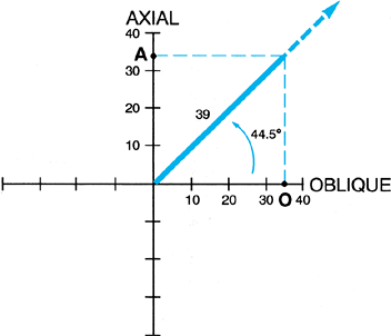
Figure 32.38. If one adds rotation to the evaluation of angular deformity, then an xyz
graph can be used to determine the orientation of the axis and magnitude of the deformity. The oblique plane deformity is calculated first in the method described. One then plots the oblique plane magnitude on the x axis and the rotational magnitude on the z or axial axis. In the example illustrated, there is a 25° varus angulation and a 25° procurvatum angulation, producing a 35° oblique plane deformity oriented 45° to the frontal plane. In addition, there is a 34° rotational deformity. This is plotted on the axial axis. The graph demonstrates a 39° angular deformity oriented at a 44.5° inclination to the transverse plane. This axis can be further qualified as oriented at 45° to the frontal plane on the transverse cut. |
either through a single hinge or sequentially. The correction requires
a hinge that is oriented not in the transverse plane but inclined, in a
vertical plane. This vertical inclined hinge will simultaneously
correct the angular and rotational deformities (Fig. 32.39).
If the osteotomy is done at the angulation-translation point,
angulation, translation, and rotation are corrected simultaneously. The
alternative, which is simpler, is to correct the angular deformity
first, then to correct the rotational deformity using a derotation
mechanism. While this method is more time consuming, it is easier for
most surgeons to understand. However, some translational correction may
be needed after derotation because of the eccentric location of the
bones within the ring. The advantage of the single-hinge method is that
no maltranslation results from the deformity correction.
 |
|
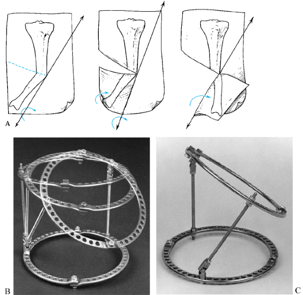
Figure 32.39. A:
Vertical inclined plane hinge. When the paper is folded with the tibia marked on it along a vertical oblique axis, the tibial diaphysis is both realigned as to its angular deformation and derotated. B: This principle can be applied to the Ilizarov apparatus. By using universal hinges, two rings can be connected by hinges at different levels. The axis of rotation is no longer parallel to the plane of the rings but rather is in a plane that is vertically oblique to the rings. C: In this simulation, the upper ring can be seen to pivot through the vertical oblique axis. Notice the position of the central bolt connecting the half rings on the moving ring relative to the central bolt on the stationary ring. In this reduced position, the central bolts are properly aligned. In the flexed position, the central bolts are rotated with respect to each other. |
principles. By producing a single osteotomy in a vertical oblique
plane, a surgeon can correct all of these deformities by sliding the
bone surfaces perpendicular to the plane of the osteotomy (27,31).
one level of angulation. Each level and each plane of deformity must be
delineated for each apex. Sometimes a single osteotomy can be used to
correct a multiapical angular
deformity,
but usually more than one osteotomy is needed. Often one of the apices
is obvious, while the other is subtle. This happens when one of the
deformities is diaphyseal and the other is juxtaarticular. Examples are
anteromedial and posterolateral bows of the tibia (Fig. 32.40).
Usually, a varus or valgus diaphyseal deformity exists with a
compensatory juxtaarticular angular deformity at the level of the
proximal tibial physis. Correction requires two osteotomies:
angulation-translation in the proximal tibia, and angulation in the
mid-diaphyseal region. These are called compensatory bowing deformities
because one deformity compensates for the other. There is usually
little deviation of the mechanical axis.
 |
|
Figure 32.40. Anteromedial tibial bow. A:
The frontal plane alignment of the tibia demonstrates an obvious varus deformity of the mid diaphysis and a subtle valgus deformity of the juxtaarticular region of the tibia. There is also a very mild distal femoral valgus and a leg-length discrepancy. B: The osteotomies were performed in the proximal metaphysis and in the mid diaphysis. The distal osteotomy is for the correction of the varus and the procurvatum deformities; the proximal osteotomy is for the correction of the juxtaarticular valgus deformity. Notice the pattern of the olive wires, which provide the necessary fulcrums and distraction points for this correction. C: The apparatus is shown in the immediate postoperative period. Each ring is oriented perpendicular to its own bone segment. The mid-diaphyseal hinge is properly located. The proximal tibial hinge was incorrectly located at the level of the osteotomy. This was one of the authors’ earliest cases before the principles of angulation plus translation for juxtaarticular deformities were completely understood. D: At the end of the correction, all of the rings are parallel and the hinges are straight. E: The AP and LAT radiographs demonstrate the realignment of the tibia on both views, as well as double level lengthening to equalize the limb length. F: The final radiograph demonstrates the realignment of the tibia with slight undercorrection of the distal angular deformity and slight overcorrection of the proximal angular deformity, which made up for the lack of translation at the proximal osteotomy. The preoperative planning of this case is illustrated in Fig. 32.44. |
 |
|
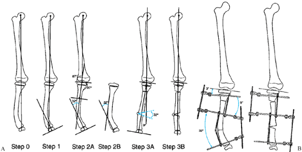
Figure 32.44. A: Multiapical angular deformity of the tibia with a normal femur. Step 0:
Draw the mechanical axis line from the center of the hip to the center of the ankle, demonstrating minimal varus mechanical axis deviation. The malalignment test was performed, demonstrating a normal distal femoral alignment. Step 1: Draw the proximal and distal tibial mechanical axis lines. Note that the intersection point is at a nondeformed level. The intersection of these two lines is not at the level of the obvious deformity. Notice that the proximal tibia also does not lie on this line. This indicates that there is a second apex of deformity. Step 2A: Draw the line perpendicular to the middle segment of the tibia and extend this line proximally and distally. This should intersect the mechanical axis of the distal tibia at the level of the true apex of deformity. Step 2B: The same center of rotation is located by the convex cortex method. Step 3A: Correct the first deformity at the level of the obvious apex. Extend the corrected distal mechanical axis line proximally. This intersects the proximal tibial mechanical line at the growth plate. This is the second apex. The second osteotomy is of angulation and translation to realign the tibia. B: The apparatus before and after correction. |
deformity that develops in soft bone, as is seen in rickets, Paget’s disease, and osteogenesis imperfecta (Fig. 32.41, Fig. 32.42 and Fig. 32.43).
Whether due to remodeling or ongoing multiple stress fractures, these
deformities demonstrate no single or double apex. While a bow can be
considered to have a single apex, realignment through the apex corrects
only the mechanical axis and does not improve the anatomic axis of the
bone. It is preferable to perform at least two osteotomies to
straighten a bowed bone. An alternative is to perform an osteotomy at a
level different from that of the apex of the bow, and to combine this
with a translational correction so as to eliminate some of the anatomic
axis deformity.
 |
|
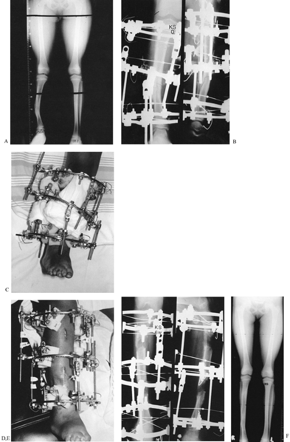
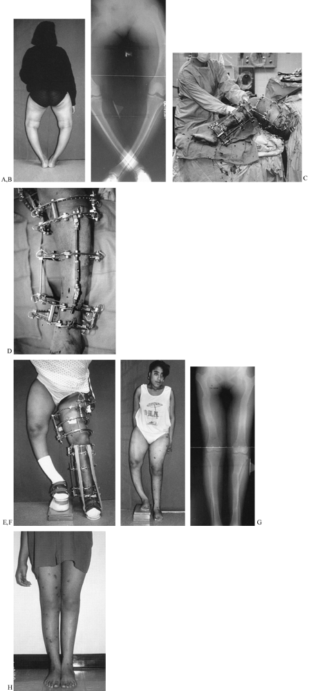
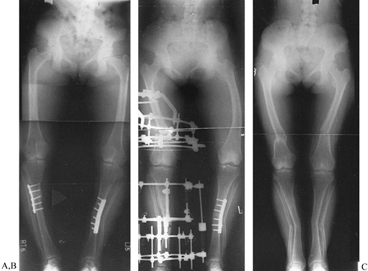
Figure 32.41. A: Back view of an 18-year-old woman with severe bowleggedness from hypophosphatemic rickets. B:
The radiographs demonstrate the severity of the preoperative deformity. Both legs do not fit on the width of a normal film, even when the legs are crossed. Notice the bowing in the femur. Notice that the bowing in the femur is diffusely distributed throughout the length of the femur, as is the bowing in the tibia. Notice also the lateral compartment joint laxity in the knee, which contributes to the varus deformity. C: The apparatus is shown during construction in the operating room. The femoral apparatus is applied first, followed by the tibial apparatus. The two devices need to be coordinated to allow at least 90° of free flexion of the knee. Care must be taken so that the most distal femoral and most proximal tibial rings do not collide. For this reason, incomplete rings (5/8 rings) open posteriorly are applied adjacent to the knee. D: The tibial apparatus from the frontal view. The hinges are locked at the measured deformity. The incision for the distal corticotomy of the tibia is shown adjacent to the hinge. There are two levels of fixation within the proximal and distal segments.E: At the completion of the realignment, all of the rings of both the femur and the tibia are parallel. Notice the axial increase in length from realignment of these severely bowed bones. F: After removal of the apparatus, the patient was left with a 10-cm leg-length discrepancy. The realigned limb stands in marked contrast to the uncorrected side. G: The second side was corrected after a 4-month hiatus. Notice that the left tibia was slightly overcorrected to try to compensate for the lateral knee joint laxity. On the right side, the proximal fibula was pulled down 1 cm to tighten the lateral knee joint. Notice that even in bipedal stance, the lateral knee joint is wider on the left than on the right leg. Notice also that the fibular head lies more distal on the right then on the left side. H: The final clinical appearance of both legs shows normal alignment with an excellent cosmetic and functional result. |
 |
|
Figure 32.42. A: A lateral photograph of the marked anterior bow (“saber shin”) deformity of the leg in a 75-year-old woman. B:
The LAT radiograph demonstrates monostotic Paget’s disease with two levels of ununited stress fractures and an intact posterior fibular strut. C: A push construct was applied to the tibia. Notice the single level of fixation in the proximal and distal tibia and three floating levels of fixation on opposite sides of the stress fractures. Anteriorly, a sliding plate suspends the three floating half-rings. The threaded rods of this plate are used to push in the apex of the deformity. On the concave side, there are two distraction rods, of which only one can be seen on the photograph. Both a knee and an ankle Dynasplint unit were used to help prevent joint contractures. D: The apparatus is shown in situ at the beginning of the deformity correction. A fibular osteotomy was performed. The posterior aspect of the two nonunions can be seen to open slightly as the combined distraction and apical translation are carried out. E: At the end of the deformity correction, there is an opening wedge at both nonunion sites. The proximal and distal tibial rings as well as the three floating half rings are all parallel. F: The apparatus was removed when a complete wall of cortical bone was seen posteriorly and when the fibula had united. This correction also equalized the patient’s leg lengths. G: The clinical appearance is excellent. |
 |
|
Figure 32.43. A:
Bilateral genu varum from varus deformities of both femurs and the right tibia. Both tibias have been previously operated on. The right tibia still has a varus deformity. The preoperative planning of the right side of this deformity was illustrated in Figure 32.23. B: A single level of osteotomy was chosen for both the tibia and the femur. One could justify two levels of osteotomy within each bone; however, since the amount of bowing in each bone was not severe, it was felt that this could be treated as a single apex angular deformity, recognizing that it truly was a multiapex angular deformity. Therefore, we chose to ignore the anatomic axis of the tibia and realign both the mechanical axis of the tibia and the joint orientation of the knee and ankle. This gives the patient a result similar to that achieved on the plated left side. The alternative would have been a combined proximal and distal tibial osteotomy, which would normalize both the anatomic and the mechanical axes of the tibia. An acute correction was performed in the femur at a level distal to the apex of the deformity, as described in Figure 32.23, to minimize the lateral indentation of the side that would result from a single-level, more proximal osteotomy at the apex. C: The result demonstrates complete realignment of the hip, knee, and ankle joint orientations, as well as the mechanical axis. On the opposite side, the osteotomy was performed slightly distal to the apex of the deformity and, therefore, a lesser amount of translation was needed. The result in terms of joint alignment and orientation is identical. |
The clue that there is more than one apex of angulation is that the
single center of rotation determined by the intersection of the
proximal and distal mechanical axis lines is at a level where there is
no “obvious” angulation (Fig. 32.44, step 1).
In multiapical deformities, there is usually one obvious (diaphyseal,
hip, or ankle) apex and one less obvious angulation apex. The obvious
apex should be corrected first. The apex of this level may be chosen
based on cortical or midbone lines, or, in the case of hip or ankle
deformities, we know the apex is at the center of the joint. Once the
first apex of angulation is corrected, it will point to the second apex.
malalignment, correct it together with the tibial or femoral varus
angulation. With conventional techniques, the head of the fibula can be
osteotomized and moved distally. By the Ilizarov method, the proximal
fibula is pulled down to tighten (even overtighten) the lateral complex
(Fig. 32.15, Fig. 32.41).
The medial collateral ligament can also be tightened by distracting the
tibia through an osteotomy proximal to the insertion of the medial
collateral ligament. To tighten the medial collateral ligament without
pulling down the patellar tendon, direct the osteotomy of the tibia
obliquely, distally, and laterally, to exit below the tibial tuberosity
(Fig. 32.15).
opening wedge, dome, closing wedge, or angular displacement
osteotomies. Both distraction and conventional methods use all of these
osteotomy types. With conventional osteotomy, the correction is
achieved acutely in the operating room; stability is achieved with
internal or external fixation. The closing wedge technique is preferred
because of the good bone-to-bone contact possible. Conventional opening
wedge methods usually require a bone graft and have a higher incidence
of nonunion. The dome osteotomy is a compromise between the opening and
closing wedge, avoiding the length loss of the closing wedge method and
offering some adjustability. The complications with these techniques
include nonunion, osteomyelitis, compartment syndrome, nerve injury,
and vascular injury (6). Accuracy
of correction is often a problem, especially with the closing wedge
technique. Even with meticulous planning, factors such as x-ray
magnification, rotated x-rays, measurement error, the thickness of the
saw blade, and the expertise of the surgeon all contribute to
inaccuracy with conventional methods (19). After the operation, there is no nonoperative way to adjust incomplete correction (15,17).
accurate. Since Ilizarov’s technique is percutaneous, there is little
risk of compartment syndrome, nerve injury, vessel injury, nonunion, or
osteomyelitis. The correction is performed either acutely for small
deformities or gradually for larger deformities (25).
Gradual distraction prevents nerve stretch injuries, as can occur in
the correction of a valgus tibial deformity. The distraction method is
as accurate as one can measure on a radiograph, perhaps the greatest
advantage of Ilizarov’s technique. Even after acute corrections,
adjustments can be made to fine-tune the correction until the exact
alignment of the limb is achieved.
correct as frontal or sagittal plane ones. More complex deformities,
including rotation, translation, and limb-length discrepancy, can all
be managed simultaneously. Multilevel and multibone corrections can be
done since there is little blood loss and the apparatus can be applied
to multiple levels and bones simultaneously. Lengthening can be
performed for small and large discrepancies, as needed, at one or more
levels. Associated problems of nonunion, contracture, and osteomyelitis
can be treated at the same time. The apparatus allows for unrestricted
weight bearing and personal hygiene; weight bearing is usually
restricted with internal fixation, and bathing is difficult if a
protective cast is used.
related to external fixation, including wearing a bulky apparatus for a
prolonged period, pin infections, muscle transfixion, loss of joint
range of motion, and pain. With proper application of the device, the
last three problems should be minimal. More recently, with the use of
half
pins instead of transfixion wires, these problems have been significantly reduced.
advantageous in treating complex deformities. Nevertheless, it still
offers many advantages even for simple deformities that have a good
conventional alternative, such as high tibial osteotomy. The decision
to use Ilizarov’s distraction method rather than a conventional
osteotomy and fixation depends on all of these factors, not the least
of which is the surgeon’s experience in the application of the
distraction osteotomy.
using hinges consists of two levels of fixation proximal and two levels
distal to the apex of the deformity (Fig. 32.45).
Each level of fixation is perpendicular to either the anatomic or the
mechanical axis of the bone fragment to which it is affixed. The hinge
connects the proximal and distal blocks of fixation, articulating
between them at the desired center of rotation for correcting the
angular deformity (23).
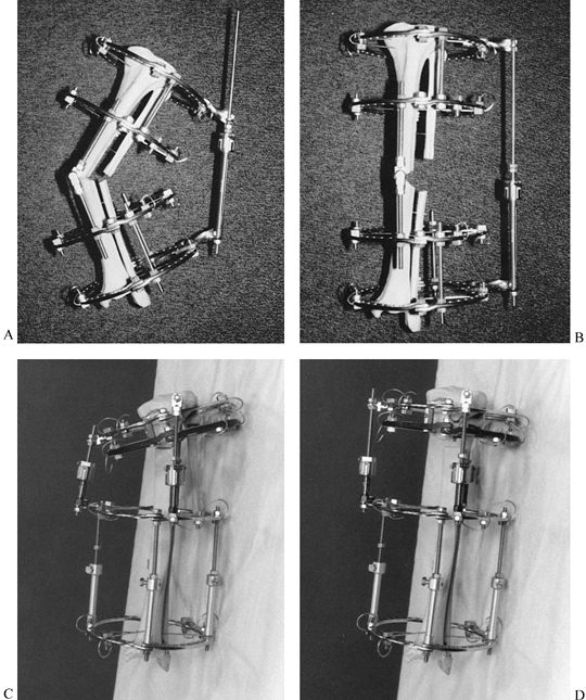 |
|
Figure 32.45. A:
Center of rotation hinge apparatus. There are two levels of fixation in each bone segment on opposite sides of the osteotomy. The rings are applied perpendicular to their respective bone segment. The hinge lies perpendicular to the ring. In this example, the hinge is applied over the apex of the deformity, with the hinge rod overlying the medial convex cortex of the tibia. On the concave aspect, there is a distraction rod connected by two twisted plates and a suspending post. The post connection to the twisted plate allows for self-adjustment of the distraction rod angle to that of the ring. B: After the correction is completed, all the rings are parallel and the hinge rods are colinear. Notice the open-wedge correction of the tibia and fibula and the change in angle between the distraction rod and the ring. C: For a juxtaarticular deformity of the tibia, the apparatus employs a translation hinge. Notice that the hinge is located over the level of the tibial physis. This is proximal to the upper ring. Two levels of fixation were achieved in each bone segment on opposite sides of the osteotomy. D: At the end of the correction there is an angulation and translation of the bone segments at the level of the osteotomy. The rings are now parallel and the hinge rod is straight. Notice again the change in orientation of the distraction rod to the rings. |
the convex side, then distraction of the concavity will lead to an
opening wedge correction (Fig. 32.34, Fig. 32.46A).
If the hinge is placed at a distance from the convex side of the apex
of the deformity, then lengthening will occur together with correction
of angular deformity (Fig. 32.46B, Fig. 32.47). Placing the hinge on the concave side of the deformity will lead to compression of the bone ends with angular correction (Fig. 32.46C, Fig. 32.48).
If the hinge is placed either proximal or distal to the level of the
osteotomy, then translation of the bone ends will occur with angular
correction during distraction of the concavity (Fig. 32.46D, Fig. 32.49).
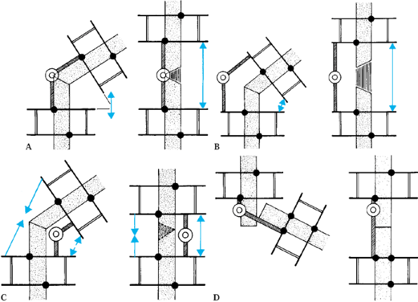 |
|
Figure 32.46. A:
Opening wedge hinge. The hinge is located at the level of the osteotomy overlying the convex cortex of the bone. Distraction of the concavity leads to an opening wedge correction without separation of the convex cortices of the bone. B: Distraction hinge. The hinge is located away from the convex cortex of the bone but still at the level of the osteotomy. Distraction of the concavity leads to simultaneous lengthening with angular correction. The regenerate has the appearance of a trapezoid, with a wider separation on the concave side than on the convex side. C: Compression hinge. If the hinge is located at the level of the osteotomy but on the concave side of the bone, distraction of the concavity will lead to compression of the bone ends. If the bone ends allow, this will produce a closing wedge type of correction. D: Translation hinge. If the hinge is located proximal or distal to the level of the osteotomy, distraction of the concavity will lead to translation of the bone ends. In this example, the hinge is located at the intersection point of the convex cortices of the two bones and, therefore, distraction of the concavity leads to correction of the angulation and translation of the bone ends. |
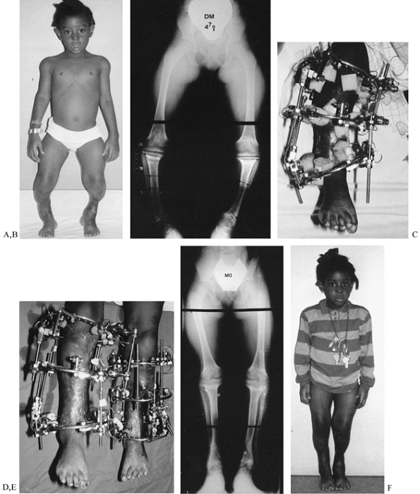 |
|
Figure 32.47. Application of distraction hinges for lengthening and correction of deformity. A:
A 5-year-old girl with bilateral genu varum and shortening due to meningococcemia septic emboli. She has skin grafts adherent to the bone and, therefore, distraction must be performed very gently. B: Standing radiographs show the deformities and the preoperative planning markings for the placement of olive wires. C: The apparatus has a hinge located lateral to the convex aspect of the osteotomy. To augment the stability of the fixation, the distal hinge has a threaded rod applied through the center of the anterior and posterior hinge point. This can be performed only with distraction hinges. D: Toward the end of the correction, notice the increased length achieved through the distraction hinges without lengthening on the hinge rods. All of the lengthening is performed by distraction of the concavity. Notice that this method is gentle on the skin and there were no skin problems. E: The final radiographs demonstrate 8 cm of lengthening of both tibias with realignment. Notice the bilateral triangular shaped tali. Both feet were plantigrade at the end of the correction. F: The final appearance of both legs at the end of the lengthening and correction of deformities. |
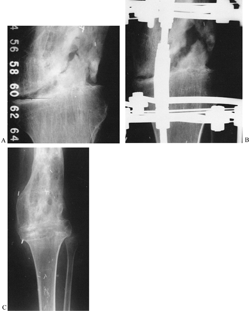 |
|
Figure 32.48. Application of compression hinge. A: Valgus deformity with nonunion of knee arthrodesis site. B:
The apparatus was applied with a hinge overlying the center of the knee joint so that distraction of the concavity would produce compression of the medial aspect of the nonunion and distraction of the lateral aspect of the nonunion. C: The final result demonstrates correction of deformity and union. |
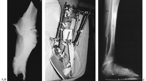 |
|
Figure 32.49. A: Application of translation hinge. Equinus malunion of ankle arthrodesis. B:
This was treated by a supramalleolar osteotomy with application of a translation hinge. The hinge was located at the level of the calcaneotibial fusion; the osteotomy was performed 3 cm proximal to that. C: Simultaneous lengthening, angulation, and translation were carried out. Notice the position of the tibia overlying the mid foot. The entire foot has translated posteriorly to give this girl a heel and to shorten the stiff forefoot, improving her ambulation. Notice the translational pattern of the trabeculae. |
level of the osteotomy to avoid any translation of the bone ends with
respect to each other, unless translation is planned as part of the
correction (23). Conversely, if translation of
the bone ends is desired, then the proper level of the hinge needs to
be selected. The level of the hinge is also governed by the bisector
line of the angular deformity (Fig. 32.50).
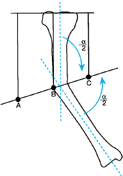 |
|
Figure 32.50. Determination of hinge placement level by the bisector concept. A, distraction hinge; B, opening wedge hinge; C, compression hinge.
|
The bone must be locked into the apparatus in such a way that the bone
ends will follow the angular correction of the rings. To create such a
constrained system, the appropriate fulcrum and distraction points must
be built in. The position of the fulcrum and distraction points is best
described as a four-point bending maneuver (Fig. 32.52).
The “rule of thumbs” is used to determine the location of the fulcrum
and distraction points for simple angular corrections without
translation of the bone ends (23,25). In coronal plane deformities, insert olive wires in the frontal plane according to the four-point bending rule of thumbs (Fig. 32.52).
For sagittal plane deformities, use transverse smooth wires in the
frontal plane at all four levels of the rule of thumbs instead of olive
wires (Fig. 32.53). Alternatively, threaded
half-pins can serve as fulcrums for either sagittal or coronal plane
deformities. It is preferable to use two olives counteropposed on the
same side as the fulcrum or distraction point whenever possible. In the
femur, threaded half-pins often substitute for olive wires.
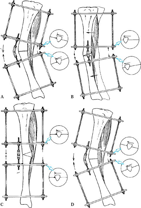 |
|
Figure 32.51. The principle of constraint of the apparatus to the bone. A,B:
If smooth wires only are used, distraction of the concavity of a deformity will lead to slippage on the smooth wires. The bone tends not to elongate with the correction but to move toward a part of the apparatus in which there is less elongation. Therefore, the bone moves from the convex side of the apparatus toward the concave side of the apparatus. This slippage leads to incomplete correction of the bone by the time the rings are in a corrected position, and it may lead to impingement of the skin against the ring on the convex side of the deformity. C,D: Applying olive wires over the apex of the deformity prevents slipping. The concave bone and soft tissues are forced to elongate. |
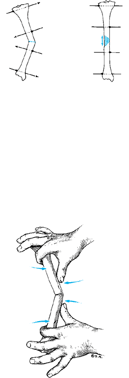 |
|
Figure 32.52.
The rule of thumbs. Four-point bending is the principle of correction in angular deformities. Olive wires are placed at the fulcrum point on opposite sides of the apex of the deformity and at the distraction points at either end of the bone. The location of the olive wires can be remembered by thinking of the four point bending rule of thumbs; the olive is located at the points where the thumbs press on the apex and the index fingers press on the ends of the bone. |
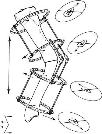 |
|
Figure 32.53.
In sagittal plane deformities, the transverse wires act to constrain the system in much the same way as olives do for frontal plane deformities. |
the olives counteropposed between blocks but on the same side of the
two levels of fixation within a block (Fig. 32.54) (25).
Therefore, the proximal two olive wires are on the same side and the
distal two olive wires are on the counteropposed side. In this pattern,
the olives act to push the bone’s distal segment from its translated
position toward the properly aligned proximal segment.
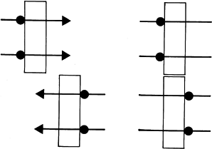 |
|
Figure 32.54. For translational deformities, the olives should be counteropposed.
|
correction using a hinge, the olive wires are placed in a modified rule
of thumbs to effect both translation and angulation (Fig. 32.55) (23).
This requires the addition of a third olive wire on the side without
the hinge. The third olive wire is the translation wire that forces the
translational correction simultaneously with the angular correction. If
half-pins are used, they act to constrain the construct, thus replacing
the need for olive wires.
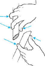 |
|
Figure 32.55.
The modified rule of thumbs helps determine the location of the olives for combined angulation translational corrections. While one fragment is held as usual between the index and thumb, the other fragment is held with the thumb and index at the same level on opposite sides of the bone and the middle finger in the previous location of the index finger. The olive pattern is illustrated in Fig. 32.46D. |
osteotomy and identify the magnitude and true plane of the deformity.
Construct an apparatus to correct the deformity. Construct two blocks
of fixation, each with two levels of fixation. Plan the spacing between
levels according to the strategy of correction. If only angular
correction is required, then make the blocks as wide as possible, with
only a handbreadth separating the blocks at the level of the deformity.
If significant lengthening is planned, the distance between blocks must
be greater to avoid skin entrapment. In this situation, the width of
each block is narrower.
deformity, perpendicular to the plane of deformity. In addition to the
plane of the hinge axis, the level of the hinge and its function must
be chosen. Place a hinge either at the level of the osteotomy or at a
different level. The latter
will
produce a translational effect during correction. Usually the hinge is
placed at the level of the deformity’s apex and the osteotomy is done
as close to that level as other considerations permit. The function of
the hinge as opening wedge or distraction will determine its distance
from the center of the ring.
the calculated magnitude of angular deformity and lock it in that
position. Place a distraction rod between adjacent rings at a point
halfway between the hinges on the opposite side of the limb. The
preconstructed frame is then ready for application.
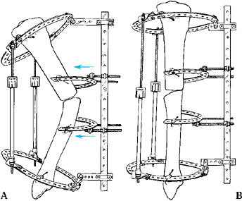 |
|
Figure 32.56. Push construct. A: The push construct is shown applied to a procurvatum deformity of the tibia, similar to the example illustrated in Fig. 32.42.
The proximal and distal rings are perpendicular to their individual bone segments. The middle half-rings are suspended from an anterior plate. The plate, connected via buckles to a perpendicular shorter plate, pivots on the ring on a hinge. The buckles allow the horizontal plates to slide up and down while the hinges allow the horizontal plate to alter its orientation to the ring as the deformity gradually corrects. The half-rings are connected by threaded rods from posts on either side of the long plate. On the concavity, there are two distraction rods connected by twisted plates and posts to allow auto-adjustment at either end. Only a single wire is needed on each of the floating half rings, and two wires are used at either end on the full ring. B: By coordinating the distraction on the concavity with the translation on the convexity, the deformity is gradually corrected. Notice that the buckles have moved toward each other on the long plate. |
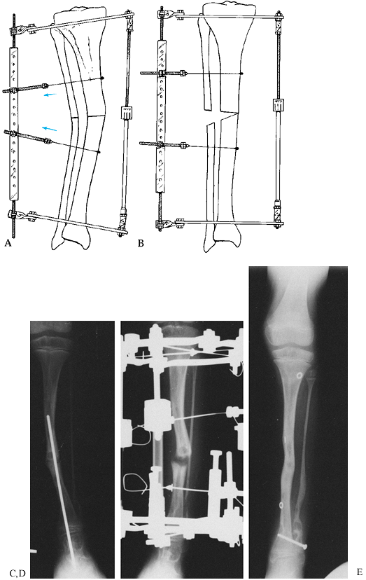 |
|
Figure 32.57. Pull construct. A:
The apparatus at the beginning of the correction, with olive wires on slotted threaded rods. The olive wires pull in the apex of the deformity, much the way the push wires push in the apex of the deformity. In the minor deformity shown, conical washers are used at each end for distraction. Alternatively, a focal hinge or twisted plate at either end could be used. B: The appearance of the construct at the end of correction. C: Preoperative AP roentgenograph of a patient whose congenital pseudoarthrosis of the tibia was previously treated by a nail and onlay grafting. Note the valgus ankle and proximal migration of the fibula. D: Distraction of the stiff pseudoarthrosis using a pull construct to correct the deformity. E: Union, lengthening, and realignment were all achieved. The fibula was transported distally. It was transfixed with a screw to keep it from proximal migration and a bone graft applied to synostose it to the tibia. It remains united 2 years later. (C, D, and E from Paley D, Catagni M, Argnani F, et al. Treatment of Congenital Pseudoarthrosis of the Tibia. Using the Ilizarov Technique. Clin Orthop 1992;280:91.) |
-
Affix the most proximal and most distal levels to a ring, and apply distraction rods on the frame’s concavity.
-
On the convex side, articulate the rings
with a long plate. The articulation on the plate acts as both a pivot
and a sliding joint. The apex of the deformity is either pushed or
pulled into the concavity. -
A push construct uses smooth wires perpendicular to the plane of the deformity (Fig. 32.56).
A pull construct uses olive wires in the plane of deformity. Connect
the push smooth wires to a translational apparatus. Connect the pull
olive wires using a slotted threaded rod translation apparatus (Fig. 32.57).
segment, this construct is less stable than the hinge construct.
Therefore, this frame should be applied only to relatively stable
pathologies such as stiff nonunions, bowing deformities with a large
resistive tension band of soft tissue on the concavity (Fig. 32.42), and bones that do not have great loads applied to them, such as the forearm.
Two levels of fixation within each bone segment articulated with hinges
and a distraction rod on the concavity are augmented by a push
construct on the apical two rings of the deformity to achieve augmented
fixation and augmented constraints on the deformity.
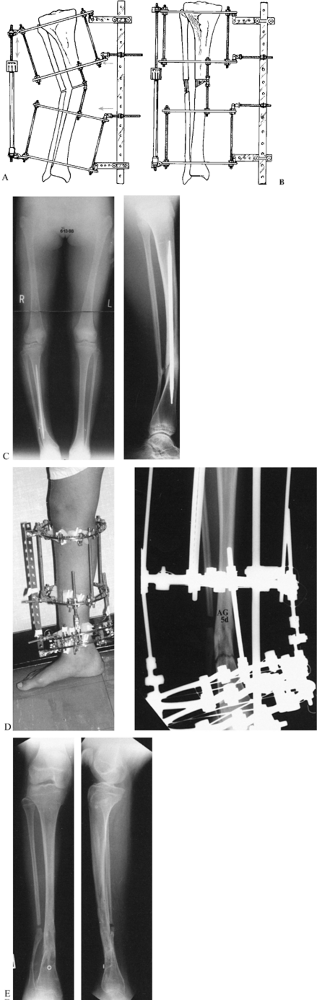 |
|
Figure 32.58. Combination hinge and push constructs. A: The strongest construct of all combines the two levels of fixation of the hinge construct with the push construct. B: The construct at the end of deformity correction. C: The construct shown in (A) and (B) was applied to a congenital pseudoarthrosis, which had malunited, in an effort to fracture the bone without an osteotomy. D:
Ilizarov calls this method metaphysealysis. It can be used to focus large concentrated forces on weak, narrow-diameter bone regions. Notice the fracture of the bone that has occurred. E: The final result, showing union and correction of the deformity. |
inclined plane hinge, while a theoretical possibility, is usually too complex to be readily applied (Fig. 32.49). Two types of rotational corrections can be achieved with the circular frame: acute and gradual.
disconnecting the frame and rotating one section with respect to the
other. This can be done at the time of surgery. Because acute
correction is too painful in most outpatient situations, a controlled
acute method is preferable. One of these methods is to angle the rods
between one ring and the other and then tighten them. If all the rods
are angled one or two holes over, then an acute derotation of one or
two holes is achieved (Fig. 32.59A, Fig. 32.59B),
resulting in 5° to 10° of derotation, depending on the ring diameter.
This can be repeated every few days until the correction is completed,
usually with minimal discomfort. An alternative method is to shift the
wire on the ring (Fig. 32.59C, Fig. 32.59D)
so as to bow each end of the wire in an opposite direction like a
pinwheel; when the wires are tensioned, the bone rotates. This method
is usually too complex, time-consuming, and painful, since all the
wires need to be loosened and retensioned.
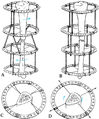 |
|
Figure 32.59. A:
Acute rotational correction can be achieved by moving the rods around the ring the same number of holes and then acutely tightening the nuts at either end of the rods, forcing the rods to become perpendicular to the ring and thus derotating the ring. B,C,D: Acute derotation can also be performed by advancing all the wires in the same direction by the same number of holes and then tensioning them acutely. This is very difficult, time consuming, and painful, and it is rarely done. |
at a set rate and rhythm determined by bone and soft-tissue
considerations. The gradual method is the safest and involves the least
amount of discomfort.
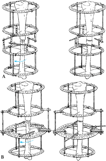 |
|
Figure 32.60. Gradual derotation can be carried out by a variety of constructs. A:
One method uses horizontal threaded rods articulating between a post on one ring and a threaded rod coming from the other ring. The threaded rod is connected by two nuts to one ring, while at the other end a buckle is attached to allow for axial support. Alternatively, a threaded rod can be connected between two posts, but this is less stable. Three of these constructs are connected around the ring. B: Another method of derotation is the ring within a ring. With this method, the proximal block is connected to the outer ring and the distal block to the inner ring. The articulation between the ring is by means of a pair of plates protruding from three or four locations. The plates are fixed to the inner ring but not to the outer ring. They sandwich the outer ring between either plate. A single horizontal threaded rod is used to motor the derotation. |
configuration’s center of rotation is at the center of these rings. If
the bone is located at the center of the ring, then
the
derotation will occur around the central axis of the bone. In most
cases, however, the bone does not lie in the center of the ring: In
both the thigh and the shank, the bone is eccentrically located within
the soft-tissue mass. To center the bone within a ring, a ring of very
large diameter would be needed, increasing the system’s instability (Fig. 32.61).
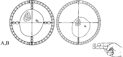 |
|
Figure 32.61. A:
The ring is normally centered around the leg so that there is a minimum of two fingerbreadths’ (3–4 cm) space between the inner edge of the ring and the skin. Notice that the center of the ring lies posterior and lateral to the center of the tibia. B: To center the ring on the bone, it would be necessary to use a much larger ring to allow a minimum of two fingerbreadths’ space between the ring and the skin. This leads to less stable fixation. |
To a lesser extent, internal rotation is associated with posterior
translation and external rotation with anterior translation. In the
femur with its anterior location, the same relationships hold.
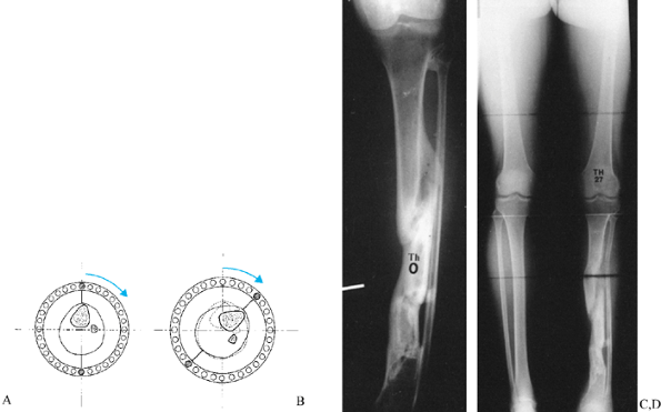 |
|
Figure 32.62. A: Rotation of a ring that is centered on the leg and not on the bone leads to (B) lateral translation of the bone. C:
This malunion required a correction of varus and rotation. There was also a lateral translational deformity. Notice that there are two lateral translations and one medial translation of the united fragments. The result is lateral translation. D: A corticotomy at the junction of the proximal and middle thirds of the tibia was performed, and the angular deformity corrected at that level. The bone was then lengthened and derotated. Because the ring was centered on the leg and not on the bone, a medial translational deformity, which can be seen, occurred. In this particular case, this was therapeutic because it realigned the translation of the tibia. Therefore, the translational effect of the derotation in some cases can be used to achieve a desired translational correction. Since the center of the ring is posterior to the tibia, internal rotation leads to medial translation, while external rotation leads to lateral translation. This deformity must be factored into the realignment of the leg, especially in large derotations. |
separate translational correction may be needed after derotation with
either a translation device or a derotation-translation device. The
former uses a translation frame modification to move the bone into the
reduced position. The latter uses the translation-rotation point to
reduce the fragments (Fig. 32.63). The
translation-rotation point is on the bisector of the center of each
bone segment. Where this bisector crosses the ring is the location of
the rotation center.
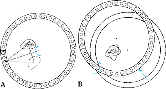 |
|
Figure 32.63. A:
To correct the translational deformity created by a derotation, one can use either conventional translational constructs or the more accurate translation rotation point. This point is located on the ring equidistant from the center of the two bone ends. The true plane of the translation must be identified, and then a point between on the line connecting the centers of the two bones is projected to the ring as the right bisector of that line. B: A threaded rod is connected between the adjacent rings at that point and the rings are derotated around that threaded rod to rotate one bone fragment into the other. This leads to reduction in the translational deformity without loss of the rotational correction. |
was discussed earlier. Translation may also be corrected independently
of angulation, either acutely or gradually. Acute translational
correction may be achieved with olive wires and acute displacement
using a wire tensioner (Fig. 32.64).
Alternatively, acute correction will occur when tensioning an arced
wire from both ends. Gradual translational correction can be achieved
using gradual distraction on olive or arced wires using slotted
threaded rods.
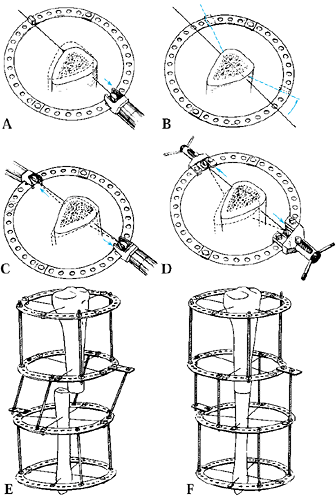 |
|
Figure 32.64. A:
Acute translational correction, which can be performed by olive or arced wires. An olive wire can be pulled from the nonolive end to translate the bone fragment. B: The same effect can be created perpendicular to the wire by using the arced wire. The wire is displaced one hole in the direction of the desired translation. C: Tensioners are applied to both sides of the wire to pull out the arc and thus displace the bone into the concavity of the arc. D: For large displacements, the original Russian wire tensioners are used. E: Another acute method of effecting a translational correction is similar to the acute rotational method by displacing the threaded rods. F: The acute translational correction is performed by tightening the nuts in the threaded rods. |
rings (Fig. 32.65).
This allows very gradual translational movement in any direction.
Unlike the rotational rods, which are oriented tangential to the ring,
the translational rods are oriented parallel to each other in the
direction of translation.
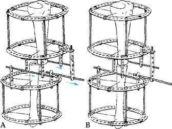 |
|
Figure 32.65. A:
Gradual translational corrections are carried out by connecting horizontal threaded rods all parallel to each other. Three of these connections are necessary. B: The end of the translational correction. |
rotation, translation, and shortening. In correcting combinations of
deformity, the order of corrections is important. Complex deformities
can be divided into two groups: those with and those without bone
segments that must translate with respect to each other. Unlike lines
on paper, segments of bone cannot slide past each other without
colliding. Therefore, any manipulation that will lead to collision of
one bone segment with another will cause obstruction and jamming of the
system.
Collision and jamming may occur when translation or rotation of bone
fragments is required as part of the correction. The propensity for
collision and jamming depends on the configuration of the bone
fragments with respect to each other and the contour of their bone
ends. Of course, a transverse osteotomy through a bone with no overlap
of the bone segments will allow movements of angulation, rotation,
translation, and lengthening without collision and damage. On the other
hand, if the two bone segments overlap, translation or angulation will
be obstructed. In such a situation, the surgeon must first lengthen the
limb and then correct angulation and translation together (Fig. 32.66, Fig. 32.67).
When there is an oblique or spiral osteotomy and rotational correction
is required, lengthening must be done first to avoid collision and
jamming of the oblique bone segments with each other.
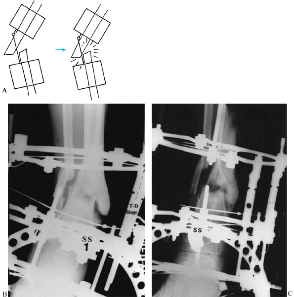 |
|
Figure 32.66. A:
When a translational correction is to be performed at the same time as an angular correction by means of a translational hinge, jamming of the bone ends may occur. B: A valgus malnonunion of the distal tibia. A translational distraction hinge is in place to correct the length, angulation, and translation simultaneously. C: Notice that the angulation was corrected but the translation was not correctable because of jamming of the bone ends. The deformity should have been distracted first to separate the bone ends, and then the hinge should have been activated. |
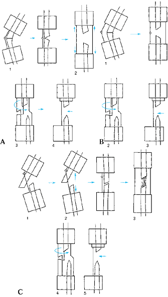 |
|
Figure 32.67.
Order of deformity correction. The order of correction depends on the risk of premature consolidation and the propensity for jamming of the bone ends. A: Order I: (1) angulation; (2) lengthening; (3) derotation; (4) translation. B: Order II: (1) simultaneous angular correction and lengthening; (2) derotation; (3) translation. C: Order III: (1) partial lengthening; (2) angulation; (3) lengthening; (4) derotation; (5) translation. |
rate of healing of the bone or the patient. In younger children, the
expected rate of healing is faster than in adults. Open-wedge
angulation correction carries a risk of premature consolidation on the
convex side; this would prevent subsequent lengthening. This risk is
small in adults but significant in children. Therefore, the order of
corrections in adults and children may be different.
whom premature consolidation is not a concern, the order of corrections
is angulation, lengthening, rotation, and translation (Fig. 32.67A).
at risk for premature consolidation, the order is angulation and
lengthening, rotation, and translation (Fig. 32.67B).
In these patients, the angulation and lengthening may be done
simultaneously using a distraction hinge or lengthening on the hinged
rods at differential rates from the distraction rods. In this
situation, some of the length and some of the angulation are corrected
simultaneously until the angular deformity or the length discrepancy is
completely corrected, leaving either residual angular or length
deformity to correct. This is followed by derotation and translation.
corrections is lengthening, angulation, remaining lengthening,
rotation, and translation (Fig. 32.67C).
translation through long segments of regenerated new bone, where the
shearing effect of these displacements can be distributed along the
soft bone and blood vessels. There is far greater shear between bone
ends of an undistracted osteotomy (leading to disruption of medullary
and periosteal tissues during translation or rotation) than there is
between bone ends that are separated by several centimeters.
translational displacement may occur during derotation of an
eccentrically located bone. This displacement may be used if both the
translational deformity and the rotational deformity are in the same
direction. In these cases, the bone ends can be rotated, thereby
correcting translation and rotation simultaneously.
rotational correction, since rotation is possible with significantly
consolidated regenerate bone. Correction of translation is difficult in
the presence of advanced consolidation. Angulation is feasible even
later than rotation in the face of advanced consolidation. Therefore,
the order of deformity correction may need to be altered if the
bone
segments show evidence of premature or advanced consolidation. In these
cases, the surgeon may want to correct translation first, derotate
next, and finally correct the angulation.
In limb lengthening, all the distraction rods can be lengthened at this
rate to create a separation of the bone fragments of 1 mm/day. In
angular correction, a calculation must be made to obtain a rate of
distraction of 1 mm/day of the osteotomy site. We use the geometric
rule of similar triangles (Fig. 32.68), which
allows us to calculate the rate of distraction of the threaded rods
that will produce a 1 mm/day distraction rate at the level of the bone (23).
As the lengthening proceeds, the rule of similar triangles must be
recalculated because the distraction rod approaches the concave aspect
of the bone. For small deformities this is inconsequential, but with
large deformities it is significant.
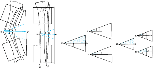 |
|
Figure 32.68. Rule of similar triangles. The rate of distraction of the distraction rod D that will produce 1 mm of opening wedge at the concave cortex of the tibia T
is calculated based on similar triangles. In the example shown, the ratio is 4:1. Therefore, it takes 4 mm of distraction at the distraction rod to produce 1 mm of opening wedge of the tibia. In contrast, the fibula lies halfway between the distraction rod and the hinge. Therefore, at 4 mm/day distraction, the fibula will lengthen 2 mm/day. Because the peroneal nerve is at the level of the fibula, it may be preferable to open the wedge relative to a 1 mm rate of the fibula rather than the tibia. |
circles (rather than triangles) that radiate around the hinge point.
The calculation of the length of arc followed by the concentric circle
at the radius R from the hinge is an
approximation of the length of time needed to correct the deformity (Fig. 32.69) (10).
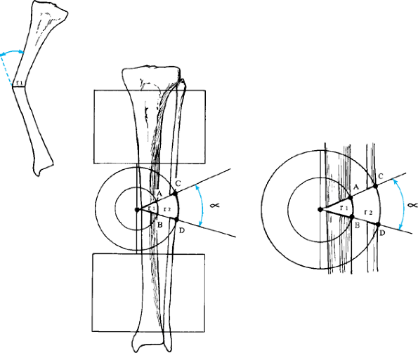 |
|
Figure 32.69.
The rule of concentric circles. Because the deformity correction is occurring around a hinge, the true pattern of correction follows the path of an arc of radius r where r is the width of the bone at the level of the osteotomy. Because the rate of correction is set to 1 mm/day at the concave cortex of the tibia, the length of the arc across the concave cortex is equal to the number of days it will take to correct the angular deformity. Arc length can be calculated as the number of degrees subtended by the arc divided by 360 times the circumference of the circle (2πr). For a deformity of magnitude α, the number of days to achieve correction of deformity is 2πrα/360. |
rate of lengthening. For example, in a contracture of the knee,
correction may be adjusted so that the sciatic nerve is distracted at a
maximum of 1 mm/day (Fig. 32.70). The calculation of the length R
is made from the center of the hinge to the sciatic nerve. Similarly,
in valgus corrections of the tibia, the peroneal nerve may be the
structure determining the rate of distraction.
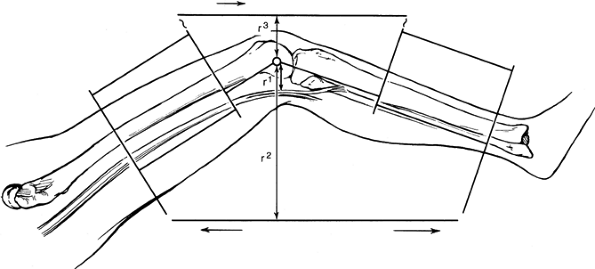 |
|
Figure 32.70.
Reciprocal rule of triangles. It is sometimes necessary to distract on one side of a deformity and compress on the other side. For example, in this knee contracture, the rate of distraction of the concave distraction rod is calculated by the rule of similar triangles. The rate of compression of the convex rod is a factor of r3 to r2, the rate of the distraction rod. In the example shown, the rate of distraction or compression is related to stretching of the most important tissue, which in this case is the sciatic nerve. The sciatic nerve is located at a distance of r1 from the center of rotation. The length r1 is used in the calculation of similar triangles. |
of distraction but also the rate of compression on the bone’s opposite
side. This can be done by the reciprocal rule of triangles (Fig. 32.71).
In most cases, distracting one side at the rate of similar triangles
and allowing the apparatus to self-adjust on the compression side
avoids any errors of rate adjustment between the two sides.
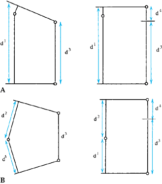 |
|
Figure 32.71.
Alternate method for calculating the treatment time for angular correction. A quick and simple method for calculating the total number of days of distraction until the rings become parallel is to subtract the length of the distraction rod between its connection point on the ring from the length of the hinge rods. A: When the hinge lies on the ring, the space between the rings is used as the length d1. B: When the hinge lies between the rings, the lengths of the limb above and below the hinge are added (d1 + d2) and then d3 is subtracted from the sum of the other two. The difference d4 is then divided by the rate of distraction of rod d3 to calculate the total treatment time. |
deformity correction is to measure the distance between the rings at
the level of the hinge and the distance between the rings at the level
of the distraction rod. The distance between rings at the hinge will
change little before and after deformity correction if no distraction
is carried out on the hinge rods. The difference between the hinge rod
width and the distraction rod width divided by the rate of correction
is an accurate approximation of the time needed for correction (Fig. 32.71).
At the end of correction, the rings should be parallel if the apparatus
was properly applied. Therefore, the difference between the distraction
rod width and the hinged rod width will eventually be zero.
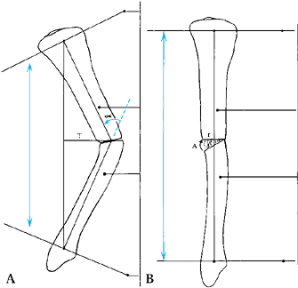 |
|
Figure 32.72. A. Coordinate the rate of apical translation with that of concavity distraction. Step 1: Use the rule of similar triangles to calculate the rate of distraction at the distraction rod. Step 2: Use the 2πrα/360 calculation to determine the number of days until complete deformity correction. Step 3:
Measure the distance for complete apical translation from the center of the bone at the level of the apex to the line connecting the center of the joint above with the center of the joint below. Step 4: Divide the total distance to be translated (T) by the number of days of correction. This will be the rate for apical translation. B. Complete correction. |
done at a rate of 0.5–1.0 mm/day. When translation is done through a
lengthy distraction gap, 1 mm/day is used; 0.5 mm/day is used when
translation is done through a narrow distraction gap or through an
undistracted osteotomy.
about 1 mm/day at the surface of the bone. The number of degrees of
rotation to keep the surface rotation rate to 1 mm/day depends on the
diameter of the bone: 12° for a 1 cm diameter bone, 6° for a 2 cm
diameter bone, 4° for a 3 cm diameter bone, and 3° for a 4 cm diameter
bone. The rate should be adjusted for small and large bones.
technique depends on the ring size. The number of degrees between
adjacent holes is equal to 360° divided by the total number of holes.
[The count should include the solid portion of the rings adjacent to
the flare (four per ring, two per half-ring).] Dividing the number of
millimeters per hole by the number of degrees per hole gives the number
of millimeters per degree of arc. Multiply this by the number of
degrees permissible for different-diameter bones to get the rate of
correction. Divide this number by three or four times per day to split
the rate into a dosed rhythm of correction. In most cases, this works
out to be 1 mm three to five times per day.
when above-average bone formation is seen. These guidelines serve to
optimize the new bone formation according to the basic biological
principles of Ilizarov (12). They must be altered in situations of hypotrophic and hypertrophic
bone formation. In the former, the rate may be cut by 25% to 50% as
needed, while in the latter the rate may be increased by similar
amounts.
scheme: *, classic article; #, review article; !, basic research
article; and +, clinical results/outcome study.
TDV, Siu D, Fisher B. The Use of Standardized Radiographs to Identify
the Deformities Associated with Osteoarthritis. In: Noble J, Galasko
CSB, eds. Recent Developments in Orthopedic Surgery. Manchester, U.K.:Manchester University Press, 1987.
GA. The Tension-Stress Effect on the Genesis and Growth of Tissues.
Part II: The Influence of the Rate and Frequency of Distraction. Clin Orthop 1989;238:263.
RP, Haertel M, Stussi E. Tibial Torsion Calculated by Computerized
Axial Tomography and Compared to Other Methods of Measurement. J Bone Joint Surg Br 1980;62:238.
KA, Pepe CL, Galloway EJ. A Mathematical Analysis of the Effect of
Flexion and Rotation on Apparent Varus/Valgus Alignment of the Knee. Orthopaedics 1990;13:861.
JW, Teitge RA, Gowda M. Preoperative Planning for the Treatment of
Nonunions and the Correction of Malunions of the Long Bones. Orthop Clin North Am 1990;21:693.
D, Chadhray M, Pirone AM, Lentz P, Kautz D. Treatment of Malunions and
Nonunions of the Femur and Tibia by Detailed Preoperative Planning and
the Ilizarov Techniques. Orthop Clin North Am 1990;21:667.
BJ, Sangeorzan BP, Hansen ST, Judd RP. Mathematically Directed
Single-Cut Osteotomy for Correction of Tibial Malunion. J Orthop Trauma 1989;3:267.
JW, Kuo KN, Andriacchi TP, Galante JO. The Influence of Walking
Mechanics and Time on the Results of Proximal Tibial Osteotomy. J Bone Joint Surg Am 1990;72:905.
has confirmed Ilizarov’s contention that small details of frame
application can make a major difference in the clinical outcome of
fractures treated by circular external fixation (1,2,8,9,10,11 and 12).
This section reviews some of the technical details of applying a
circular external fixator, using Ilizarov’s technique and modifications
of it. Modern circular external fixation techniques utilize both wires
and pins at multiple levels for optimum fixation of osseous fragments.
frame can slide back and forth along a limb unless two or more wires
are used at each level of fixation. For maximum stability, the two
wires should cross each other at a right angle. Unfortunately, anatomic
constraints (neurovascular structures, muscles, and tendons) limit a
surgeon’s ability to insert wires crossing at 90° within a bone at most
locations. For this reason, transfixion wires usually end up crossing
each other at a more acute angle, diminishing fixator stability.
Therefore, to enhance fixation, a surgeon must often use more than two
wires at each level or alternatively must insert additional wires
oblique to, or away from, the ring’s plane.
systems use wires with beads (“olive wires”) that abut the bone to
prevent the bone from sliding along the wire, at least in the direction
of the bead (Fig. 32.73). Olive wires can also be used to pull bone segments and to reduce fractures and for other applications.
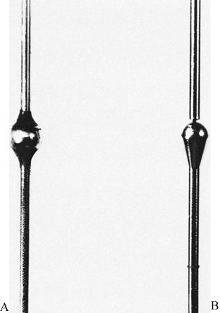 |
|
Figure 32.73. Beaded wires. Original design (A) and modified design (B).
|
-
Avoid synovial transfixion when possible.
-
Do not impale tendons.
-
Penetrate muscles at their maximum functional length.
application of an external fixator, means that the position of a nearby
joint must change as the wire passes through the flexor and extensor
muscle groups. For example, when inserting a wire from anterolateral to
posteromedial in the distal femoral metaphysis, flex the knee to 90°
before inserting the wire into the quadriceps, and push the wire
straight down to the femoral cortex (Fig. 32.74) (14).
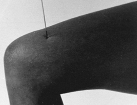 |
|
Figure 32.74. Flex the adjacent joint when inserting wires into the extensor surface.
|
-
Drive the wire through the bone with a
power drill. As soon as the wire emerges through the far cortex, stop
drilling, extend the knee, and hammer the wire through the opposite
side of the limb with the hamstrings at maximum stretch. To drive a
wire through soft tissue with a mallet, either tap the wire’s end or
grasp the wire with pliers and strike the pliers with a mallet (Fig. 32.75).![]() Figure 32.75. Tap the wire through the soft tissues on the limb’s far side with a pliers and mallet.
Figure 32.75. Tap the wire through the soft tissues on the limb’s far side with a pliers and mallet. -
When inserting a wire into the lower leg,
plantar-flex the foot when transfixing the anterior compartment, invert
the foot when inserting wires into the peroneal muscles, and dorsiflex
the foot during triceps surae impalement (13,15).
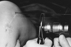
wires through transfixed muscle; the position of the skin is another
matter. Flexing the knee during femoral wire insertion pulls the lower
anterior thigh skin distally, while the posterior skin slides a bit
proximally. Transfixion of anterior thigh skin during flexion (the
optimum position for quadriceps impalement) might cause a limitation of
knee extension, impeding ambulation and perhaps leading to a knee
flexion contracture. For this reason, before wire insertion, the skin
must be shifted in a direction appropriate to adjacent joint motion. In
determining which way to move the skin before inserting a wire,
consider the following:
-
When lengthening a limb, some redundant
or loose skin and subcutaneous tissue should overlie the corticotomy
site, where stretching will be greatest. Thus, when inserting
supracondylar wires into the femur for lengthening through a distal
corticotomy, pull the skin and subcutaneous tissues proximally during
wire penetration, and at the same time flex and extend the knee to
shift the muscles as previously described (Fig. 32.76). Likewise, displace the skin and subcutaneous tissues distally when applying the ring proximal to the proposed osteotomy site.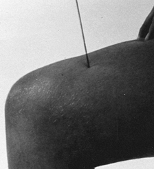 Figure 32.76. Pull the skin proximally for lengthening before wire insertion.
 -
When correcting a deformity by an opening
wedge corticotomy, the skin and soft tissues should be loose, if
possible, on the deformity’s concave side. In the case of a tibia varus
correction, for example, shift the medial subcutaneous tissues downward
during proximal ring application and upward while the distal ring is
being applied. -
Whenever possible, select wire placement
locations that normally have limited skin movement during flexion or
extension of an adjacent joint, usually along the medial and lateral
lines of a limb.
successful circular external skeletal fixation. When inserting a wire,
avoid necrosis of tissue caused either by “wrapping up” around the
wire’s tip or by thermal injury caused by heat build-up during drilling.
-
Although transfixion wires are smooth,
they have bayonet tips that can cause damage while spinning within soft
tissues. For this reason, when inserting a wire, push it straight down
through the soft tissues to the bone (Fig. 32.77). Begin drilling when the wire’s tip is at the bone’s surface.![]() Figure 32.77. Hold the wire with a wet gauze to stabilize it during insertion.
Figure 32.77. Hold the wire with a wet gauze to stabilize it during insertion. -
Stop drilling intermittently to prevent
heat build-up. Cool the wire with irrigating solution during drilling,
especially when penetrating dense cortical bone. As soon as the wire
emerges from the bone’s opposite side, stop drilling, and drive the
wire through the limb’s soft tissues with a mallet and pliers (6). -
If a wire emerges with blackened bone on
its tip, then the wire has burnt the bone; remove the wire, cool it,
and reinsert it elsewhere. Do not use a burnt bone hole for external
skeletal fixation, as the bone around the hole has no resistance to
invading microbes.
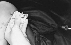
the wire’s flexibility may cause the wire to bend, reducing the
accuracy of wire placement. While it seems appropriate to “chuck up”
the wire closer to its tip, such a maneuver may nick the wire, leading
to early breakage if the nick is located anywhere between the fixation
bolts. Instead, grasp the wire with a 2×2 gauze pad soaked in
antibiotic solution close to its blunt end and stabilize the spinning
wire.
-
After inserting a wire, but before
attaching it to a frame, check the wire–skin interface for evidence of
tension while the limb is in its functional position—the knee extended,
the ankle at neutral, and so forth. Skin tension creates a ridge of
flesh on one side of a wire (Fig. 32.78A). To
eliminate this tension on the side of a wire tip, withdraw the wire tip
slowly (with the pliers-and-mallet technique) until the point drops
below the skin surface (Fig. 32.78B). Shift the skin to a more neutral location and advance the wire until it penetrates the skin in an improved position (Fig. 32.78C).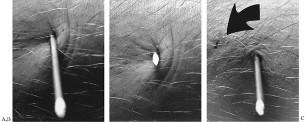 Figure 32.78. Dealing with skin tension. A: Tension at a wire site. B: Withdraw the wire and allow the skin to shift. C: Drive the wire through the skin in a new position.
 -
If skin tension exists on the insertion side of a wire (Fig. 32.79A), snap off the wire’s blunt end obliquely to create a point (Fig. 32.79B) and advance the wire to below the skin surface by the pliers-and-mallet method on the limb’s far side (Fig. 32.79C). Adjust the skin with the point below the skin (Fig. 32.79D). Tap the wire back through the skin after a skin-position adjustment (Fig. 32.79E).
![]() Figure 32.79. Tension on the insertion side of a wire. A: Tension between two wires on the insertion side. B: Withdraw the wire and make a point on the blunt end. C: Pull the point below skin level. D: Adjust skin with the point below the skin. E: Advance the wire through the skin in a new position.
Figure 32.79. Tension on the insertion side of a wire. A: Tension between two wires on the insertion side. B: Withdraw the wire and make a point on the blunt end. C: Pull the point below skin level. D: Adjust skin with the point below the skin. E: Advance the wire through the skin in a new position. -
If an olive wire causes skin tension on
the side of the limb opposite the olive, simply back out the wire until
the tip drops below the skin surface and make the correction described
above. If the tension is on the olive side of the wire, enlarge the
skin incision for the wire to relieve the tension.
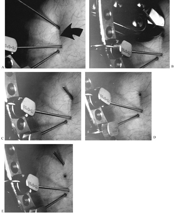
wire–skin interface tension: modifying fixation after an acute
deformity correction. For example, when a fixator is applied to manage
a congenital coxa vara, part of the correction can be done immediately
after subtrochanteric osteotomy. The skin, however, may be pulled
distally on the transfixion wires as a valgus subtrochanteric angle is
established. If this occurs, shift the skin upward after the correction
and insert additional wires or pins before removing the ones causing
the skin tension. Release any residual skin tension with a scalpel.
straighten any bend or curve in the wire. Soft tissues on either side
of a bent wire may suddenly be stretched during wire tensioning,
causing intense postoperative pain. Thereafter, the stretched soft
tissues can become necrotic, providing nutrition for microorganisms
that enter the limb through the wire holes. For this reason, do not
bend a wire toward the frame during fixation; instead, use washers,
posts, and other hardware to build up to and capture the wire where it
lies (Fig. 32.80).
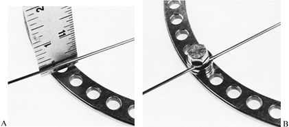 |
|
Figure 32.80. Securing a wire off the plane of a ring. A: Wire 1/8 in. off plane of ring. B: Wire secured with washers and a bolt.
|
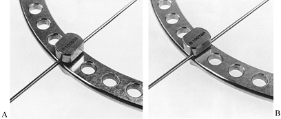 |
|
Figure 32.81. Securing a wire on the plane of a ring. A: Cannulated fixation bolt used for wire over the center of a hole. B: Grooved fixation bolt for wire between two holes.
|
configuration depends to a considerable extent on the amount of tension
on the wires. Tensioning a wire axially stiffens it mechanically; with
enough tension, a transfixion wire behaves like a stiff pin. Moreover,
a deflection load applied to a tensioned wire (by weight bearing, for
example) increases wire tension even further, enhancing wire stiffness
and resistance to additional deflection. When the deflection load is
released, the wire usually springs back to its original position,
although some permanent plastic deformation might occur. This
mechanical behavior of tension wires stimulates osteogenesis in a
bone-defect site, according to Ilizarov.
-
Tension a wire with either a
spring-loaded wire tensioner or by the fixation bolt method (winding
the wire around its own fixation bolt). When using these methods, be
sure to fix the wire securely to the ring on the limb’s opposite side.
A smooth wire can be tensioned on either side of the limb, but an olive
wire cannot. If the olive wire is meant to serve as a stabilizing
element in the assembly, fasten the wire to the ring on the olive side,
with the olive firmly abutting the bone. If the olive is to pull a bone
fragment into position before fixation, do not secure the olive side of
the wire until the maneuver is completed. -
A spring-loaded dynometric wire tensioner (Fig. 32.82)
is simple to use; both the barrel-shaped and pliers-shaped models are
calibrated. Tension the wire to between 100 and 130 kg on a full ring,
and to about 90 kg when the wire is spanning an open ring or on a pair
of posts elevated from a ring’s plane.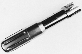 Figure 32.82. Spring-loaded wire tensioner.
 -
With the fixation bolt method (Fig. 32.83),
the wire is twisted around its own fixation bolt, tensioning it. The
maneuver requires two hands, one for the nut and the other for the
bolt. Have an assistant hold the ring stable.![]() Figure 32.83. Manual wire tensioning. A: Initial position. B: Final position.
Figure 32.83. Manual wire tensioning. A: Initial position. B: Final position. -
After fixing the wire to the ring on the
opposite side, tighten the nut until the wire is loosely gripped. Next,
rotate the fixation bolt and its nut together, twisting the wire 90°
around its own fixation bolt. Because the wire displaces slightly with
this method, try to displace
P.1074P.1075P.1076
the wire slightly during initial fixation so that it will be straight through the tissues when tensioning is complete.
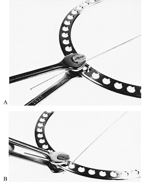
inserted without regard to cross-sectional anatomy. In 1981 I published
a “zone system” atlas for pin placement to help ensure safe application
of Hoffman pins, and I now use this atlas for inserting transfixion
wires (3). Other atlases are also available for this same purpose.
Secured With Anteroposterior Wires, And These Wires Are Attached To A
Large, Thick, Curved Plate Surrounding The Patient’s hip and pelvic
area (14). The patient must use a special bed
that incorporates a cut-out mattress to allow the posterior portion of
the frame to be suspended while the patient is flat on her back.
basic problems. First, the bulk of the soft tissues causes
difficulties, especially posteriorly, in the buttock. Second, the
neurovascular bundles—especially the superficial femoral artery—can be
damaged during wire insertion. The vessel is medial to the femur in its
proximal third and posterior to the bone in the thigh’s distal third. A
safe practice is to mark the location of the vessel after palpating the
femoral pulse. Third, the sciatic nerve prevents direct AP wire
insertion. The proximal wires must cross at a fairly narrow angle in
the upper thigh.
-
When inserting wires into the proximal
femur, mark the skin with the hip ring arch in an overcorrected
(compensated) position, higher anteriorly and laterally. During femoral
lengthening, the femur tends to angulate into varus with the apex of
the deformity anterolateral. To correct this problem, the arch must be
applied in a position that anticipates such a deformity. As lengthening
proceeds, the arch is gradually rotated downward, becoming
progressively more perpendicular to the bone’s mechanical axis during
elongation. -
Insert the first olive wire from
anteromedial to posterolateral two fingerbreadths lateral to the
femoral artery. Insert a second olive wire from back to front, 15°
medial to the first wire. The posterior olive on this wire prevents the
entire frame from displacing anteriorly while the patient lies in bed.
A third wire is often inserted between the first two. Push all three of
the proximal femoral wires through the soft tissues down to bone
without drilling, and tap the wires through the soft tissues with
pliers and mallet once the tip emerges through the opposite cortex. -
To stabilize a hip during femoral
lengthening—especially a hip that might sublux or dislocate—it may be
necessary to insert wires into the supraacetabular or iliac portion of
the pelvis. Leave these wires in place (not allowing movement) until
lengthening is complete. Thereafter, the wires are removed and hip
motion is commenced. -
When an unstable deformity is in the
middle third of the femur, a four-ring configuration may be necessary,
with two rings above the deformity and two rings below it. -
For the distal femur, insert wires into
either the transverse or the coronal plane. When selecting the
transverse plane, cross the wires at an angle of no less than 60°.
Likewise, insert olives from both directions for enhanced stability. In
many situations, the distal femur can be stabilized with wires in the
coronal plane; such wires permit greater freedom of knee motion than do
wires that impale the hamstrings and the quadriceps.
lengthening, one ring with two crossed wires and a supplementary drop
wire is used proximally, and a similar combination is used distally (15).
The stretched soft tissues help stabilize the limb. More complex
problems, such as a mobile synovial pseudarthrosis of the mid tibia,
require far more stable configurations using three, four, or even more
rings. Likewise, a deformity correction at two levels requires at least
three rings.
incorporates a wire that passes through the fibular head and into the
tibia to prevent subluxation of the proximal tibia–fibula joint during
lengthening or deformity correction. A second wire through the tibia
crosses the fibula wire, paralleling the medial face of the tibia. A
third transverse drop wire is inserted across the tibia into the
location used for skeletal traction. Additional wires are inserted as
needed for greater stability. Distally, the fibula must usually be
incorporated into the configuration with a distal fibulotibial wire.
Additional crossed wires in the distal tibia complete the mounting. The
strategic placement of the olives on these wires depends on the goal of
fixator application. The principles of olive-wire placement were
discussed earlier in this section.
Diameter Of The Wires, The Number Of Wires, The Angles Between The
Wires, The Direction Of Wire Insertion, The Plane Of The Wires, And The
Method Of Fixing The Wires To Their Support Ring.
the patient, the stiffness of the deformity, and the amount of
osteoporosis present. In general, younger patients require smaller
wires (1.5 mm) than older patients. The stiffer the deformity, the
larger the diameter of the wire (up to 2.0 mm) required.
deformity influence the number of wires selected. Usually, two crossed
wires are inserted into the tubercle of the calcaneus, subtending an
angle of about 60° between them. Use this configuration when correcting
a deformity of the os calcis, such as equinus or calcaneus. When merely
holding the bone to prevent development of equinus during tibial
lengthening, use a single transverse wire. More than two wires may be
necessary with marked osteoporosis. Keep the plane of the wires
parallel to the plantar surface of the heel.
be inserted. When correcting an equinus, insert both olive wires from
the posterior part of the heel toward the forefoot. When correcting a
cavus or calcaneus deformity, insert the olive wires from the forepart
of the foot toward the heel. When correcting a forefoot adduction
deformity, keep both olive wires on the medial side of the heel. When a
valgus of the heel is being corrected, place the olive on the lateral
side of the foot. In combined deformities such as talipes equinovarus,
the position of the olives is determined by the nature of the pathology.
location of the wires within the calcaneus. When overcoming equinus,
place the wires high in the tuber of the calcaneus to ensure good bone
stock plantarward of the wires. When correcting a cavocalcaneal
deformity, insert the wires lower in the bone to ensure a maximum stock
of osseous tissues cephalad to the wires.
nature of the problem. To overcome forefoot adduction, keep the olive
on the medial side of the foot; to correct forefoot abduction, place an
olive on the foot’s outer edge.
and fifth metatarsals, passing under the necks of the second, third,
and fourth. In certain circumstances, it may be necessary to insert
additional wires into other metatarsal bones, especially when
correcting a severe supination deformity. Pass these wires from the
plantar surface of the foot out through the neck of the third or fourth
metatarsal, exiting in the dorsolateral surface of the foot.
to correct an adductovarus foot. The first and third points of force
application (olives) are on the medial side of the calcaneus and first
metatarsal, respectively. Place the counterpressure olive wire on the
lateral side of the cuboid (or talar neck or other midfoot bone).
Can Be Secured With Three Wires Each. To Insert Wires Through The
Proximal Humerus, Abduct The Arm 90° and externally rotate it 20°.
Drive olive wires from both the anterior and posterior directions. The
third wire is a drop wire off the plane of the ring.
the frontal plane, one from the lateral supracondylar ridge and one
from the medial supracondylar ridge (Fig. 32.84).
A drop wire (perpendicular to the bone’s axis) completes the
configuration. Extend the elbow when inserting wires anteriorly and
flex the elbow when inserting wires in the posterior side of the limb.
When a humeral mounting requires three levels of fixation, wires
crossing in the mid-humeral area should be inserted with regard for the
location of the neurovascular bundles, especially the radial nerve.
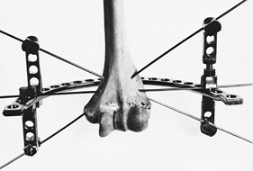 |
|
Figure 32.84. Distal humeral fixation with wires crossing in the coronal plane.
|
anterior lower-arm skin moves proximally while the posterior skin moves
distally; with elbow extension, these tissues move in the opposite
directions. Between the flexor and extensor surfaces, however, a fairly
stable tissue plane exists, around which the upward-downward movement
of the anterior and posterior tissues revolves. This plane of limited
skin movement lies along the medial and lateral supracondylar ridges of
the humerus, an ideal location for transfixion wire placement.
Unfortunately, the distal humerus flattens and widens at the elbow. Two
supracondylar transfixion wires (in the same transverse plane) will not
have enough of an angle between them for stable fixation; it is better
to cross the wires in the frontal plane.
-
Insert the wires into both epicondyles,
exiting the humerus proximally at the medial and lateral supracondylar
ridges. Take care not to transfix either the ulnar or radial nerves. A
third wire straight across from one supracondylar ridge to the other
completes the mounting. -
After all wires are in place, flex and
extend the elbow: there should be no block in either direction. A
mechanical block to full extension means that one or more wires has
entered the olecranon fossa of the distal humerus; such a wire must be
repositioned.
pathology. In some cases, the two forearm bones are secured together
with wires transfixing both the radius and the ulna. In other
mountings, each bone has its own separate fixator, with one frame
rotating within the other. Transfixion wires are particularly dangerous
in the forearm. Consult a cross-sectional anatomy atlas at the time of
wire insertion.
bone fixation. In this way, muscle impalement with transfixion pins or
wires is avoided.
-
Avoid creating a cantilever system with
pins perpendicular to the bone. Instead, our half-pins are splayed out
in different directions and different planes, with some inserted
obliquely into each bone segment (Fig. 32.85).![]() Figure 32.85. Rancho mounting with divergent titanium half-pins.
Figure 32.85. Rancho mounting with divergent titanium half-pins. -
Furthermore, try to mount the half-pins
as circumferentially around the bone as possible, attempting to gain
purchase where the osseous surface is located subcutaneously (Fig. 32.86).
The tibia and ulna are particularly suited to this type of mounting,
because these bones are subcutaneous through their length (5).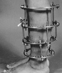 Figure 32.86. Rancho mounting with contoured ring sizing.
 -
The femur and humerus have subcutaneous
surfaces proximally and distally. For juxtaarticular mountings,
continue to use wires. Three or four wires can be easily inserted into
fragments that are unsuitable for half- or full-threaded pins.
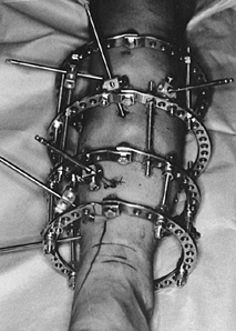
particularly well tolerated by both bone and soft tissues. If a
titanium pin site does become septic, we rarely observe
the
extensive inflammatory reaction (involving adjacent portions of the
limb) that we have noted with steel implants. Occasionally, a threaded
titanium pin becomes strongly bonded to bone, suggesting bone-to-metal
bonding similar to the type of fixation that may occur with titanium
total joint implants.
correcting deformities with titanium half-pin configurations, more pin
bending than one would expect with stainless-steel half-pins is noted.
Therefore, use 5 mm titanium pins for tibial and humeral mountings and
6 mm titanium pins in the femur. For substantial lengthenings, steel
pins have proven superior because of the added stiffness.
First, whenever a rotational deformity requires gradual correction, a
circular external fixator is the only apparatus that allows
counterrotation of the configuration’s sections. Second, a circular
frame permits application of hinges and distractors anywhere around the
circumference of a bone (Fig. 32.87). In this
way, a hinge axis can be placed wherever needed to produce the desired
bone-fragment angulation. Third, a circular fixator gives the option of
using wires—especially olive wires—when needed for interfragmentary
compression, reduction of fractures, or juxtaarticular fragment
fixation.
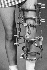 |
|
Figure 32.87. Rancho mounting with titanium pins for managing complex deformities.
|
pin technique is needed to ensure long-term fixation. When inserting
half-pins, take the following measures, which should be used for
routine external skeletal fixation as well (3,4 and 5):
-
After making the skin incision, use a mosquito clamp to spread the tissues down to the bone (Fig. 32.88).
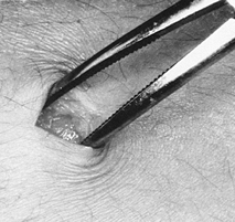 Figure 32.88. Spreading tissues with a clamp.
 -
Next, use a joker or narrow periosteal elevator to elevate the periosteum from the bone at the pin site (Fig. 32.89). This measure reduces periosteal damage caused by the spinning drill bit.
![]() Figure 32.89. Elevating the periosteum with a “joker” before pin insertion.
Figure 32.89. Elevating the periosteum with a “joker” before pin insertion. -
Use a drill sleeve and trocar with tangs
(or points) that can be driven into the bone, ensuring both stability
of the sleeve and less interposed soft tissues during drilling (Fig. 32.90).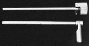 Figure 32.90. Sleeve and trocar system for pin insertion.
 -
Irrigate the drill bit with a cold irrigating solution during drilling.
-
Use a stop-and-start drilling motion to prevent the drill bit tip from overheating (7).
-
When penetrating dense cortical bone,
periodically remove the drill bit from the sleeve and wipe out bone
chaff from the flutes—another measure to prevent overheating. -
Use a depth gauge and insert a properly sized half-pin with a hand-held driver.
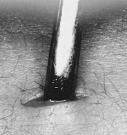
Since we have been using half-pins for our mountings, problems with
physical therapy (inhibition of muscle and joint action by wires) and
pin sepsis have greatly improved (Fig. 32.92, Fig. 32.93) (6).
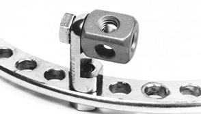 |
|
Figure 32.91. The cube used for variable-angle pin insertion.
|
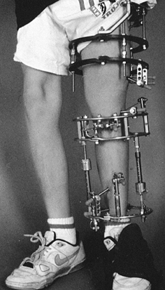 |
|
Figure 32.92. Rancho mounting for femoral and tibial lengthening. A wire is used for this patient’s hypoplastic fibular head.
|
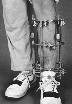 |
|
Figure 32.93. Rancho titanium pin mounting for bone transport. Notice the use of full pins in a location where no muscles are impaled.
|
scheme: *, classic article; #, review article; !, basic research
article; and +, clinical results/outcome study.
GA. The Tension-Stress Effect on the Genesis and Growth of Tissues:
Part I. The Influence of Stability of Fixation and Soft-Tissue
Preservation. Clin Orthop 1989;238:249.
GA. The Tension-Stress Effect on the Genesis and Growth of Tissues:
Part II. The Influence of the Rate and Frequency of Distraction. Clin Orthop 1989;239:263.
small-diameter wires with external frames, G. A. Ilizarov in Kurgan,
Siberia, was foremost in the development of techniques to treat a
variety of orthopaedic problems, including fractures, nonunions, and
deformities, using an innovative modular circular external fixator with
tensioned wires. This section discusses the use of the Ilizarov method
in the management of acute fractures and their complications.
occurred in the 1980s, foremost of which is the shift toward half-pin
frames and maintenance of the frame in place until union occurs in
unstable fractures. The benefits of axial micromotion for fracture
healing and bone remodeling have been well documented, leading to the
techniques of dynamization and staged dismantling of half-pin fixators
to improve fracture healing (3,7).
and biplaner fixators in the axial direction, while maintaining
approximately equal stiffness to bending and torsional loads (4,13).
These mechanical characteristics allow the beneficial effects of axial
micromotion without the deleterious effects of torsional and
translational shear.
Other factors influencing frame stiffness are size, number, and
location of the rings; divergence of the transfixing wires; use of
olive wires; and distraction or compressive loads at the fracture or
nonunion site (1,4,8,15).
Intrinsic biomechanical factors unique to each patient include weight,
cortical continuity, and integrity of the soft tissues.
analysis of fracture deformities has recently served as the basis for a
new generation of external skeletal fixators that, in their most basic
form, consist of two rings connected
to
each other by six struts. The struts can be manually lengthened or
shortened in accordance with a pattern determined by a computer program
that calculates the displacement of fragments secured (with pins and
wires) to the rings. The coordinate information is determined by
precise measurements from properly oriented x-ray views of the limb.
The Taylor Spatial Frame is the first of such devices (14).
of the upper and lower extremities is common in Russia and parts of
Western Europe, and increasingly in North America (7).
Metaphyseal fractures may have extension into the articular and
diaphyseal regions, greatly increasing the complexity of their
management. To define better these complex injuries and to clarify
treatment options, a new classification scheme (Fig. 32.94)
is offered. The main metaphyseal injury is characterized as stable (S),
unstable (U), or with diaphyseal extension (D). The three subgroups are
0, for absence of intraarticular extension; 1, for nondisplaced (2 mm
or less) intraarticular extension; and 2, for displaced (more than 2
mm) intraarticular extension.
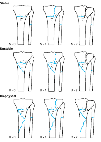 |
|
Figure 32.94. SUD classification of metaphyseal fractures accounting for increasing degrees of instability and intraarticular extension.
|
stabilization by intramedullary fixation. Treatment options are limited
to closed methods, pin external fixation, tensioned-wire external
fixation, and open reduction and internal fixation.
toward external fixation and away from open reduction. On the other
hand, with progression from subgroup 0 to subgroup 2, open reduction
becomes indicated. Acceptable reduction of the intraarticular portion
of the fracture complex must be obtained. If reduction of the
intraarticular portion of the fracture to less than 2 mm is not
obtained with traction, recommend open reduction and internal fixation.
The diaphyseal extension in type D fractures makes open stabilization
an extensive procedure. For type D-2 fractures, perform an open
reduction with limited internal fixation of the articular segments with
cancellous screws, and then neutralize the metaphyseal and diaphyseal
regions with external fixation. This method cannot make up for poor
articular reduction, however.
not alter basic treatment guidelines. However, a type III wound,
especially IIIB, favors stabilization with an external fixator. Less
exposure is needed if performing a limited open reduction and external
fixation, decreasing the amount of soft-tissue dissection, and limiting
local vascular injury.
possible with a circular external fixator. Because the wires are
tensioned and supported circumferentially, a “trampoline” of fixation
is provided (Fig. 32.95). Spanning the knee or
ankle for 4 to 6 weeks is necessary on occasion, especially with
elevation of the joint surface and bone grafting. Fixation is rigid
enough to allow early motion and partial weight bearing.
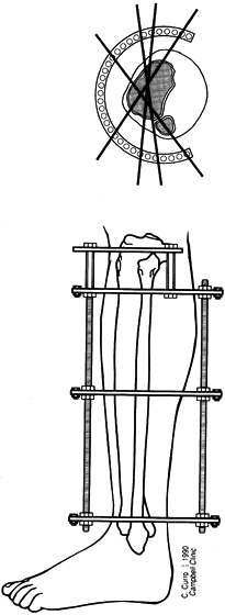 |
|
Figure 32.95.
Fixation of a tibial plateau fracture with three to four wires in subchondral bone provides a “trampoline” of support for articular fragments. |
indication for the Ilizarov method in acute trauma. The unstable
fracture, soft-tissue defect, and bone loss are all managed
successfully with one device and method. The first step in the
management of these complex fractures is to determine if the limb is
salvageable. A dysvascular, insensate extremity does not function
better than a prosthetic limb. Other relative indications for circular
fixation in acute trauma are open fractures, unstable closed fractures,
and fractures with compartment syndrome.
Accurate apposition and alignment at the time of initial application of
a simpler trauma frame is easier than the use of articulated frames
with subsequent reduction. Most fractures can be treated to union in
the external fixator, but those
of lower energy and more stability can be converted to functional bracing as healing of soft tissue allows.
preoperative planning. Assembling frames preoperatively greatly reduces
intraoperative time.
-
Obtain full-length anteroposterior (AP)
and lateral x-ray films of the limb, including the joint above and that
below. These full-length radiographs are used to select rods of proper
length and approximate ring location. -
Determine ring size on the uninjured extremity. Two fingerbreadths’ (2–3 cm) clearance is necessary for tibial mountings (Fig. 32.96), and two or three fingerbreadths’ (about 3 to 6 cm) clearance is necessary for the femur (Fig. 32.97). Rings that are too large cannot
P.1084
support the transfixing wires adequately, and they impair osteogenesis (6).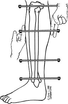 Figure 32.96. Standard clearance for a typical tibial mounting with the frame aligned with the tibial crest is 2 to 3 cm.
![]() Figure 32.97. Adequate soft-tissue clearance of a typical femoral mounting, with more space provided posteriorly.
Figure 32.97. Adequate soft-tissue clearance of a typical femoral mounting, with more space provided posteriorly. -
Because of the anatomic constraints of safe wire placement, 90° divergence is usually unobtainable (5,6,10).
A second level of fixation in each segment improves the frames’
stiffness to AP bending and torsion. Use two rings on large fragments,
and a ring and drop post for smaller fragments.

-
Accomplish fixation to the proximal femur
by half-pins attached to femoral arch bars. Connect these arch bars to
the remainder of the construct by rods and offset brackets. Make the
most proximal arch bar a short arc to prevent interference with the
abdomen when the hip is flexed. -
The entire lower extremity can be treated with a simple cylindrical frame from mid femur to the ankle, as shown in Figure 32.98.
The thigh dictates ring size, which is usually one or two sizes larger
than that normally used for the tibia. Make the frame parallel to the
tibia on AP and lateral views. Center the femur at the level of the
patella and align it in anatomic valgus with respect to the frame.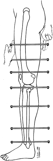 Figure 32.98. Entire lower extremity treated with a cylindrical frame with ring size dictated by the diameter of the mid thigh.
 -
When the frame is confined to the femur, use a 5/8 ring as the distal femoral ring to allow full flexion at the knee (Fig. 32.99). This 5/8
ring may be attached to a complete ring with heavy-weight sockets and
may be made more resistant to deformity when tensioned wires are
applied to the open section ring. The most proximal ring in a tibial
mounting can be a 5/8 ring attached to a complete ring, allowing maximal flexion and providing two levels of fixation (Fig. 32.100).![]() Figure 32.99. Femoral mounting using a 5/8 ring to allow full knee flexion.
Figure 32.99. Femoral mounting using a 5/8 ring to allow full knee flexion.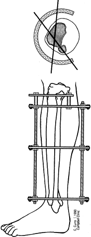 Figure 32.100. Tibial mounting using a 5/8 ring to allow full knee flexion.
 -
Include the foot in the frame for open fractures to prevent contractures and soft-tissue motion at the fracture site (2).
Pilon fractures may require foot fixation for fracture stability.
Remove the foot frame after soft-tis-sue healing, unless it is
necessary for fracture stability. With injury to the peroneal nerve or
anterior and lateral compartments, consider temporary incorporation of
the foot to prevent equinus contracture. A stable foot mounting
consists of two half-rings joined by plates with threaded extremities (Fig. 32.101).
These special plates prevent the foot frame from distorting when the
wires are tensioned. Usually the same size of half-rings are used for
the tibial frame and for the foot frame.![]() Figure 32.101. Foot mounting using two half-rings coupled by two plates with threaded extremities.
Figure 32.101. Foot mounting using two half-rings coupled by two plates with threaded extremities. -
Select the frame size to allow 2 to 3 cm of clearance between the inner edges of rings and skin (11).
Swelling and dependent edema create late changes in extremity
dimensions and must be anticipated. More clearance is needed
posteriorly for the lower extremity, and the femur requires more room
for swelling than the leg. Figure 32.96 and Figure 32.97 show typical clearances for tibial and femoral frames.
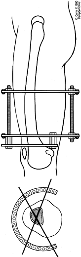
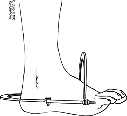
-
The Omega ring or ring with curved
extremities is useful for the proximal humeral mountings, decreasing
soft-tissue irritation and providing relatively more holes for the
critical low-divergence mountings of the proximal humerus (Fig. 32.102).
The safe angle between pins or wires is relatively small for short
fragments, requiring two wires for fixation on the ring and a wire
below or above the others. At the level of the distal humerus, the 5/8 ring allows full elbow flexion (Fig. 32.103).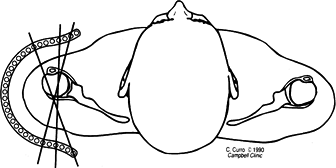 Figure 32.102. Aerial view of the shoulder, demonstrating an omega ring for proximal humeral fixation.
![]() Figure 32.103. Lateral view of the elbow with a 5/8 ring at the level of the epicondyles to allow full elbow flexion.
Figure 32.103. Lateral view of the elbow with a 5/8 ring at the level of the epicondyles to allow full elbow flexion. -
On a forearm mounting, a 5/8
ring may be used on the dorsum of the proximal forearm to allow full
elbow flexion. Provide fixation of the distal humerus by mediolateral
wires in a short arc in the coronal plane, fixed to posts above and
below the ring (Fig. 32.104). Fix the proximal humerus with anterior posterior wires in a small arc in the transverse plane.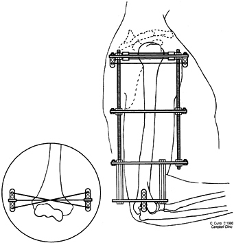 Figure 32.104. Humeral mounting showing anteroposterior fixation of the proximal fragment and mediolateral fixation of the distal fragment. (Inset) Short arc of fixation achieved with drop posts above and below the ring.
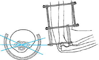
-
Position the patient supine on a fracture
table with traction placed through an os calcis pin. Place the injured
extremity in the 90°–90° intramedullary nailing position (Fig. 32.105) or straight traction in the heel-to-toe position.![]() Figure 32.105. Supine position for application of external fixation or tibial nailing.
Figure 32.105. Supine position for application of external fixation or tibial nailing. -
Elevate the buttocks support on the
fracture table on the injured side, placing the extremity in neutral
rotation with the patella pointing straight toward the ceiling (Fig. 32.106), allowing true AP and lateral orthogonal x-ray imaging.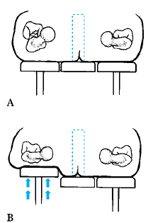 Figure 32.106. A: Supine position on the fracture table. B: Use of buttock support to internally rotate proximal limb.
 -
Alternatively, place the patient on a radiolucent table extension using the external fixator for traction and reduction.
-
Longitudinal traction reduces most fractures to within 10° or 15° of anatomic alignment.
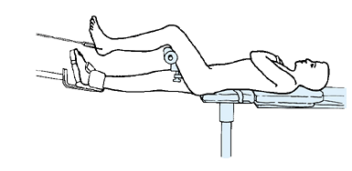
experience, has been unnecessary. Avoid excessive or prolonged traction
to prevent neurologic or vascular injury.
-
After prepping and draping the extremity,
disconnect the ring connection bolts on one side of the preassembled
frame and swing the frame open. Place the frame around the extremity
and reassemble it, with adequate soft-tissue clearance and with
coupling bolts aligned parallel to the crest of the tibia in AP and
lateral planes (Fig. 32.107).![]() Figure 32.107.
Figure 32.107.
Reference position of Ilizarov frame parallel to crest on
anteroposterior (AP) and lateral views, with connecting bolts
superimposed on AP view. -
To use this frame to treat the fracture in Figure 32.108A, hold the frame in this position with proximal and distal transverse reference wires placed parallel to the knee and ankle (Fig. 32.108B).
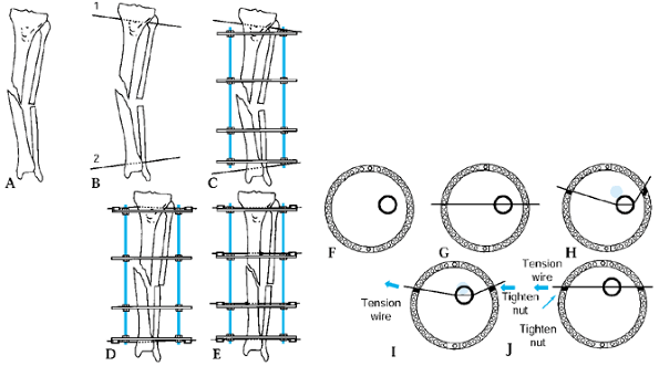 Figure 32.108. A: Unreduced diaphyseal fracture. B:
Proximal and distal coronal plane reference wires inserted parallel to
the joint at the proximal and distal extent of proposed frame. C: Ilizarov trauma frame “clamshelled” around the leg. D: Reference wires tensioned with slight residual deformity. E: Residual deformity corrected with arched olive wire technique.Parts F through J: show a cross section demonstrating the arched olive wire technique of residual deformity correction. F: Unreduced fracture fragments. G: An olive wire is inserted into one fragment. H:
Arch the olive wire the amount necessary to reduce the fragment on the
lateral view, and attach it loosely to the ring with wire fixation
bolts. I: Slowly tension the wire until the fragment is reduced on the AP view with the trailing nut subsequently tightened. J: Further tension the wire to achieve final correction of AP displacement, and then tighten the leading nut. -
As the wires are secured to the frame and tension is applied (Fig. 32.108C), further correction of the fracture in the coronal plane is achieved (Fig. 32.108D).
-
An alternative method for these initial
steps is to suspend the frame with ordinary suction tubing placed
around the extremity and secured to the frame with towel clips.
Eccentrically cant the proximal and distal rings until they are
parallel to the knee and ankle joints. After secure fixation with at
least two wires to the proximal and distal rings, bring these two rings
back parallel to their counterparts in the center of the frame, further
reducing the fracture.
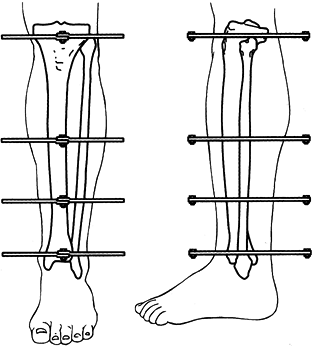
-
Use image intensification to verify
adequate reduction. To compensate for parallax curves on the image
intensifier, place an olive wire longitudinally on the extremity as an
alignment guide to confirm the reduction. -
After adequate correction is obtained in
this plane, secure the wire to the frame on the olive side. If further
correction is needed in the sagittal plane, connect the olive wire in
an arched fashion (Fig. 32.108H). As the wire is tensioned, final correction is achieved (Fig. 32.108I, Fig. 32.108J). -
Eliminate any residual distraction (Fig. 32.109).
![]() Figure 32.109. Place the fracture under compression if axially stable, to eliminate residual distraction.
Figure 32.109. Place the fracture under compression if axially stable, to eliminate residual distraction. -
In rare cases, two olive wires placed
from opposite sides perpendicular to the fracture plane can reduce and
compress the fracture (Fig. 32.110). This
pattern of wire placement may not always be safe. In such a case, treat
these fractures with lag screw fixation followed by external fixator
placement (Fig. 32.111).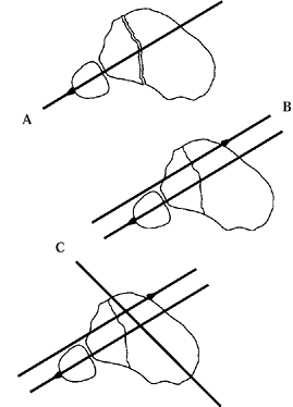 Figure 32.110. A: In an unusual case, a minimally displaced articular fracture is amenable to reduction and fixation with opposing olive wires. B: Opposing olive wire. C: Additional wires are necessary for stability.
![]() Figure 32.111. A: A more universal technique of open reduction and limited internal fixation with a lag screw than that shown in Figure 32.110. B: The plane of fixation provided by subsequent wires. C: Divergence—and thus stability—are maximized within anatomic limits.
Figure 32.111. A: A more universal technique of open reduction and limited internal fixation with a lag screw than that shown in Figure 32.110. B: The plane of fixation provided by subsequent wires. C: Divergence—and thus stability—are maximized within anatomic limits. -
Use axial computed tomography (CT) scans in preoperative planning to help determine the more appropriate method.
-
We usually avoid interfragmentary screws
or wires in the diaphyseal region, as interfragmentary fixation in the
diaphyseal region is counterproductive to the axial flexibility of the
Ilizarov external fixator; ideally, this promotes secondary fracture
healing. I avoid interfragmentary screws or wires in the diaphysis
because I have experienced delayed unions and nonunions with their use. -
Maintain distraction to achieve as much reduction as ligamentataxis provides (Fig. 32.112).
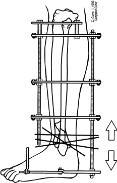 Figure 32.112. Place pilon fractures under gentle traction after fixation of the proximal tibia and the foot.
 -
Elevate depressed articular fragments and fill large subchondral voids with autogenous graft.
-
Maintain interfragmentary reduction with
wires, which are subsequently attached to the dummy ring after that
ring is translated into position (Fig. 32.113). Tension the wires and relieve any excessive traction.![]() Figure 32.113. After reduction and interfragmentary fixation with Ilizarov wires, attach the wires to a ring and add tension.
Figure 32.113. After reduction and interfragmentary fixation with Ilizarov wires, attach the wires to a ring and add tension. -
Protect pilon and plateau fractures requiring bone grafting for 4 to 6 weeks by constructs spanning the joint.
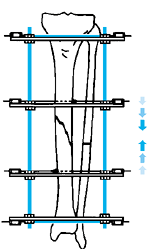
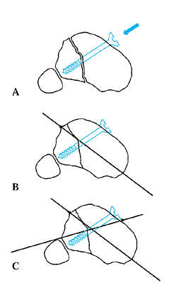
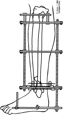
circular tensioned wire fixators. Typical fracture frames are made up
of four threaded rods linking four complete rings. Temporary removal of
one rod allows 180° access to the leg for bone grafting delayed unions
or for vascular access for free flaps (Fig. 32.114).
Removal of the anteriolateral rod allows access to the dorsalis pedis
artery, and removal of the posteromedial rod allows access to the
posterior tibialis artery.
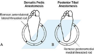 |
|
Figure 32.114. A:
Axial view of the limb showing 180° access to the anterolateral surface if a single anterolateral rod is removed for a rotation flap or free flap with the anterior tibial artery as donor. B: Axial view of limb showing 180° access to the posteromedial surface if a single posteromedial rod is removed for a rotation flap or free flap with the posterior tibial artery as donor. |
external fixator for the primary treatment. Conventional treatment
consists of debridement and delayed coverage
with
a rotation or free flap and possible internal or external fixation
followed by autogenous bone grafting. Using a tensioned wire fixator,
the wound undergoes the same serial debridement of all necrotic tissue (Fig. 32.115); if there is no exposed bone, exposed muscle can be covered with a split-thickness skin graft (Fig. 32.116). Later, the bone defect can be filled by performing a corticotomy and bone transport (Fig. 32.116).
The tendency of soft tissue to move with the transported bone, and the
normal tendency of split-thickness grafts to contract, fill in the
soft-tissue and bone defects, eliminating the need for rotation or free
flaps. If less than 2 cm of vascularized bone is exposed after
debridement, consider further shortening of fragment ends to avoid the
necessity for flap coverage. Then a simple skin graft can be used as
described previously.
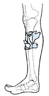 |
|
Figure 32.115. Open tibial fracture with devitalized bone, muscle, and skin.
|
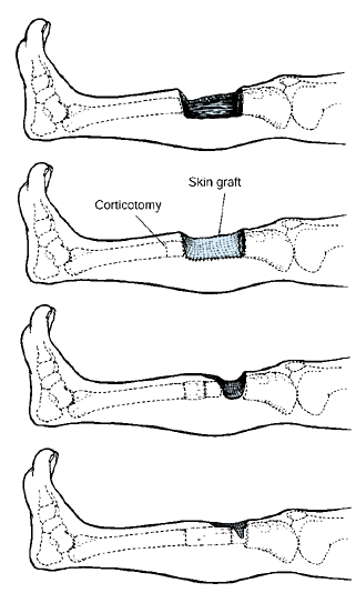 |
|
Figure 32.116. A: Open fracture following debridement, with bone loss but no exposed bone. B:
Split-thickness skin grafting of the soft-tissue defect and corticotomy in preparation for bone transport to obliterate the bone defect. C: Subsequent bone transport with regenerate bone filling the bone defect. D: Completion of transport and obliteration of bone defect. |
Although Ilizarov recommended a metaphyseal corticotomy for transport,
diaphyseal corticotomy and transport of shorter fragments has also been
successful.
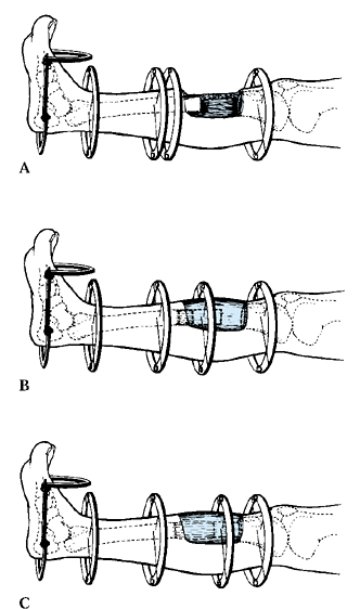 |
|
Figure 32.117. A: Open tibial fracture following debridement, with exposed viable bone requiring a rotation or free flap. B: Bone transport through the flap with formation of regenerate bone. C: Completion of transport with obliteration of the bone defect.
|
fixation, acute neurovascular injury with transfixion wires is rare. In
the immediate postoperative period, an unusually painful wire should be
suspected of passing through a larger nerve and should be removed. Late
neurovascular injury is exceedingly rare unless bone transport is
performed or there is gross motion between bone fragments. This usually
occurs during a reconstruction rather than with simple immobilization
of a fracture. Flexion contractures of the knee and ankle occur less
frequently with fracture treatment than with lengthening and can be
prevented by active exercises and weight bearing in the frame.
wires is uncomfortable for patients. Anesthetics are usually required.
Swelling and dependent edema must be anticipated with circumferential
external fixators; anterior soft-tissue clearance need not be as great
as posterior. The rings can be quite close to the anterior thigh on the
initial femoral mounting because dependent edema distends posteriorly.
Few patients can sleep in positions other than supine with a femoral
frame. For a typical adult tibial application with a distance of 36 cm
between proximal and distal rings, the frame shifts 2 cm if the frame
is canted only 3°.
-
Accurately position the frame before it
is attached to bone with tensioned wires. Place proximal and distal
reference wires at the most proximal and distal points of attachment of
the frame using an image intensifier (12). -
Insert reference wires in the coronal
plane parallel to the joint, and attach the frame to these wires,
establishing sufficient soft-tissue clearance at each end. Insert
subsequent wires between these two extremes, further constraining the
bone frame construct. -
If skin impinges on the frame near the
end of treatment, slip thin pieces of cardboard, with a slot for the
wires, between the skin and the frame. This prevents pressure necrosis
against the edge of the rings by increasing the area of contact (Fig. 32.118, Fig. 32.119). If skin impinges
P.1092
on the frame early in the treatment, frame modification is almost
always necessary. If problems exist at several rings but only along a
short arc segment of each ring, shift the frame toward the impingement
by reattaching all wire fixation bolts in new holes away from the
impingement. If the skin impinges on a single ring, modify that ring by
introducing two short plates between the ends of the half-rings,
creating an “ellipse” oriented with its major axis toward the
impingement (Fig. 32.120). Alternatively, use a saw to remove a segment of a ring if it will not affect stability.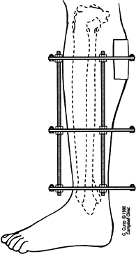 Figure 32.118. Soft-tissue impingement on an Ilizarov ring.
![]() Figure 32.119. Pressure is decreased over the metal ring by using a thin cardboard shim as a temporizing measure late in treatment.
Figure 32.119. Pressure is decreased over the metal ring by using a thin cardboard shim as a temporizing measure late in treatment.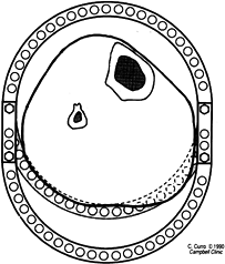 Figure 32.120. Standard ring extended by two short plates to create an ellipse, eliminating impingement of skin on the ring.
 -
Salvage major problems of circumferential
impingement at several levels by constructing a larger frame around the
first frame. Position the rings of this larger frame at exactly the
same levels. Straighten curled wire ends and attach wires to the outer
frame at both ends. Loosen the wire fixation bolts on the smaller
frame, and disassemble the smaller frame. Cannulated wire fixation
bolts from the smaller frame may be taped against the new frame to
prevent them from moving about. This modification can be performed
without loosening wires or losing reduction.
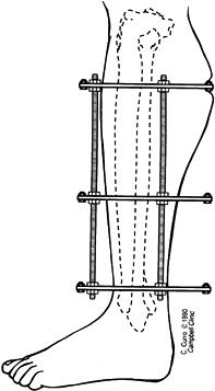
scheme: *, classic article; #, review article; !, basic research
article; and +, clinical results/outcome study.
J, Johnson E, Harp JH. Local Bone Transportation for Treatment of
Intercalary Defects by the Ilizarov Technique: Biomechanical and
Clinical Considerations. Clin Orthop 1989;243:71.
CC. Staged Reconstruction of Complex Open Tibial Fractures Using
Hoffmann External Fixation: Clinical Decisions and Dilemmas. Clin Orthop 1983;178:130.
D. The Biomechanics of the Ilizarov External Fixator. Ilizarov
Techniques for the Treatment of Nonunions, Bone Defects, Osteomyelitis,
Fractures, Adult Limb Length Discrepancy and Deformity. Washington, DC,
May 16–18, 1988.
branch of orthopaedic surgery that deals with the treatment of trauma
residuals. Indeed, Ilizarov’s techniques for causing new bone formation
within a widening distraction gap now offer patients the hope of having
an injured limb restored to normal in ways never before thought
possible (7,9,10,11 and 12).
Skeletal defects, for example, can be eliminated without the need for
bone grafting. Many types of nonunions can be stimulated to unite by
gradual distraction of the fragment ends. Malunions of all sorts can be
corrected, and posttraumatic limb shortening can be overcome.
idea of the nature of the pathologic process responsible for the
patient’s problem. For example, a nonunion of long bone may be
atrophic, hypertrophic, or a true synovial pseudarthrosis; the
treatment plan differs for each type of failed bone healing (6). A malunion in valgus or varus may also have a rotational component and malalignment of the mechanical axis as well. See Chapter 26 for more details.
treatment of nonunions, malunions, and posttraumatic shortening with
circular fixation devices.
by pain on motion of the nonunion and a feeling of resistance to manual
deformation at the fracture site. Roentgenograms of a stiff nonunion
reveal proliferative callus growing out from the fragments on both
sides of the fracture line.
examination of the fracture site. The patient often experiences little
or no pain. On roentgenograms, the fracture site may show either the
features associated with an atrophic nonunion (no evidence of callus
formation) or the characteristics of a synovial pseudarthrosis
(rounding-off and sclerosis of the bone ends).
together into the same category may seem, at first, unusual. However,
both types of nonunions demonstrate similar difficulties with healing
and require exploration and bone grafting of the nonunion site at the
time an external fixator is applied. In an atrophic nonunion, the
surgery focuses on freshening up the atrophic bone ends and removing
any nonviable tissue from the fracture site. A synovial pseudarthrosis
requires resection of the synovium and pseudocapsule, removal of the
fibrocartilage covering the bones ends, and reopening of the
intramedullary canals.
nonunions—usually heal with stable interfragmentary compression. If the
nonunion is transverse (perpendicular to the bone’s longitudinal axis),
compression with either external or internal fixation will stimulate
union. Many nonunions, however, are oblique and often combined with
malalignment of the bone fragments in angulation, rotation,
displacement (of the mechanical axes), and shortening. When any or all
of these deformities are associated with a nonunion, the Ilizarov
method permits gradual correction of all deformities, either
simultaneously or in succession. In many cases, gradual distraction
of a hypertrophic fibrous nonunion will stimulate osteogenesis in a
manner similar to the new bone formation within a widening distraction
gap. Before distraction, however, the nonunion site must be compressed
7 to 14 days, a procedure that Ilizarov claims stimulates the
bone-growth process.
oligotrophic nonunions. He performs a corticotomy of the involved bone
at a site where the surrounding soft tissues are healthy, then
gradually transports the intercalary segment through the limb. This
strategy is followed even when there is no segmental defect or
shortening. For this reason, the regenerate new bone at the corticotomy
site is often no more than 1 or 2 mm long. Nevertheless, Ilizarov
claims
good results with this tactic, based on two principles: first, the
corticotomy increases the limb’s local vascularity (a stimulus to
healing); and second, the corticotomy serves to decrease the lever arm
at the nonunion site by creating a temporary floating segment (between
the corticotomy and the nonunion). This floating segment will more
readily unite at the nonunion site under the influence of compression.
We prefer to bone graft atrophic non-unions and use the circular
fixator to eliminate shear forces at the nonunion site by using
counterpulling olive wires above and below a nonunion with an obliquity
of greater than 30°.
true plane of the deformity as well as the displacement of the
deformity’s apex from the original mechanical axis of the bone.
Likewise, determine the true angle and plane of the deformity, the
amount of rotational malalignment, and the direction and magnitude of
any displacement of the fragments by applying the principles described
by Paley and Tetsworth in the earlier section, Deformity Correction by
the Ilizarov Technique. An appropriate configuration must be designed
to correct the deformities and in the end achieve interfragmentary
compression across the nonunion. Likewise, determine if the shortening
is a result of angulation or the consequence of a true loss of limb
length.
the bone in the projection that demonstrates the maximum angulation.
Cut out the tracing, transect it through the apex of the deformity, and
straighten it out. Measure the length of the corrected cutout and
compare it to a comparable roentgenogram of the contralateral limb.
limbs in the same projection, using the view that maximizes the angular
deformity on the injured side. Draw a line on the convex side of the
deformity from a fixed landmark on the bone’s proximal end (such as the
corner of the joint line) to the apex of the deformity. Draw a second
line from the apex of the deformity along the deformity’s convex edge
to a landmark on the opposite edge of the bone (such as the tip of the
medial malleolus). Add the lengths of these two lines together, and
compare the sum to the length of a line from the same landmark on the
uninvolved limb. If there is no true shortening of the bone, then the
length of the convex side of the deformed bone should equal the length
on the corresponding side of the normal bone. If it does not,
lengthening will be needed.
perpendicular to the bone segment attached to it. In this way, the
fixator configuration mimics the deformity. In actual practice, a
mounting should exaggerate the deformity, with the rings tilted
slightly into the deformity’s concavity. During correction, resistant
soft tissues deform the wires, causing the bone fragments to lag behind
the rings during movement of the frame; the wires or pins of the
configuration will bend as the rings displace faster than the bone
fragments.
place a pair of hinges at the level of the apex of the angular
deformity. Arrange this pair of hinges so that their central bolts form
an imaginary line perpendicular to the plane of the deformity. The
distance of this imaginary line from the apex of the bone’s deformity
depends on how much lengthening must accompany the angular correction.
If, for example, eliminating the angulation results in normal limb
length, then the imaginary rotation axis of the hinges should
correspond exactly to the apex of the deformity (Fig. 32.121).
In this manner, the regenerate bone resulting from the deformity
correction will fill an “opening wedge” triangular gap. If, on the
other hand, substantial lengthening is needed, moving the
configuration’s axis of rotation away from the deformity’s apex along a
line that bisects the deformity results in a trapezoid-shaped gap
between the bone ends when the deformity is fully corrected (Fig. 32.122).
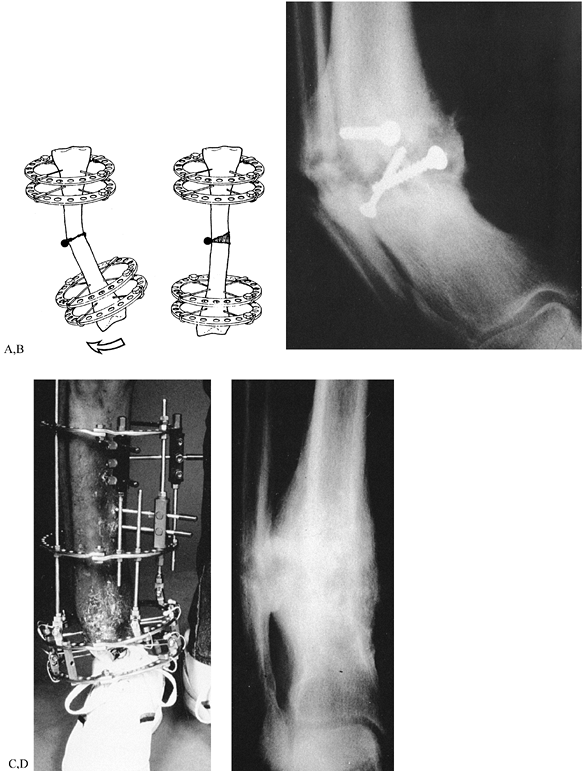 |
|
Figure 32.121. Correction of angulation. A: Scheme of correction. The black dot is the axis of rotation of the configuration. B: Severe varus deformity with hypertrophic nonunion. C: Configuration for correction. D: New bone formation during distraction and correction.
|
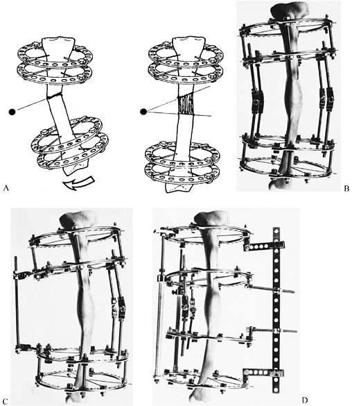 |
|
Figure 32.122. Correction of angulation with simultaneous lengthening. A: Scheme of correction. The black dot is the axis of rotation for the configuration. B: Standard method of correcting a deformity by lengthening the hinges on the concave side of the deformity. C: Less stable configuration with a distractor attached with two twisted plates. D: Configuration for stiff nonunion using a pusher mechanism.
|
common combination—the axis of rotation for the configuration’s hinges
are not on the bisector line of the deformity’s angle, but at a point
corresponding to the intersection of the mechanical axes of the bone
fragments (Fig. 32.123). If lengthening is
required along with correction of angulation and displacement, move
this rotation point a distance away from the bone that is proportional
to the lengthening needed.
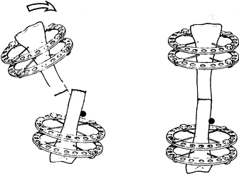 |
|
Figure 32.123. Scheme of correcting angulation and displacement. The black dot is the axis of rotation for the configuration.
|
mechanical axis. Moreover, the two main fracture fragments are often
not along the same weight-bearing line, neven when the overall
alignment of the limb is satisfactory (Fig. 32.124).
In this situation, longitudinal compression with an external fixator
(or by weight bearing) is likely to retard, not enhance, bone healing.
The fixator will either hold the bone fragments apart if the frame is
rigid (Fig. 32.125) or permit excessive shear
at the nonunion site if the frame is dynamic, especially if the
obliquity of the nonunion exceeds 30°.
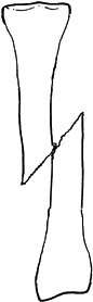 |
|
Figure 32.124. Scheme of oblique nonunion with displacement and shortening.
|
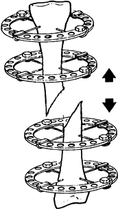 |
|
Figure 32.125. Lengthening an oblique nonunion may increase the distraction gap.
|
realign the fracture fragments, making their mechanical axes colinear,
and obtain interfragmentary (usually side-to-side) compression of the
nonunion. This combination of interfragmentary compression, axial
realignment, and stability is well known to surgeons who use plates and
screws to treat nonunions. When an external skeletal fixator is used,
the reduction must be as good as that achieved with a plate and screws.
realignment of the fracture fragments must occur gradually, using the
apparatus to achieve reduction. Often, a push configuration using long
plates in the mounting is needed to apply sufficient force on the
deformity’s apex.
corrected while the patient is anesthetized, a maneuver that simplifies
the frame considerably. When performing the manual correction, do not
create a triangular gap on the deformity’s concave side, as that will
never be able to contribute to osseous healing.
length equals that of the contralateral side, and when the nonunion is
transverse: simple axial compression will promote healing. With
increasing obliquity of the nonunion site, modify the configuration to
neutralize shear forces. Obtain interfragmentary compression by
inserting counterpulling olive wires that traverse the limb from
opposite directions (Fig. 32.126). Insert these
wires either through the site of the nonunion itself or at some
distance above and below it. Ilizarov recommends placing the wires
through an oblique nonunion if there has been no history of sepsis.
Clearly, such wires not only ensure interfragmentary compression but
also help stabilize the nonunion that they cross.
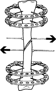 |
|
Figure 32.126. Lengthening must be combined with interfragmentary compression, shown here with counterpulling olive wires.
|
lines in the sagittal plane, since the wires enter and exit the limb on
its medial and lateral sides. When a nonunion is in the coronal plane,
however, interfragmentary compression with olive wires would require
the wires to enter or exit the limb in the anteroposterior direction.
In most anatomic locations, such wires can be dangerous. For this
reason, achieve interfragmentary compression of oblique coronal plane
nonunions by inserting wires mediolaterally into each fragment and
attaching the wires to rings or half-rings (Fig. 32.127).
Connect these rings to the rest of the configuration in a manner that
permits front-to-back interfragmentary compression at the nonunion
site. If necessary, incorporate one or two long plates in the
configuration to serve as a base for pushing and pulling the rings.
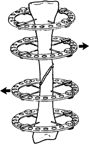 |
|
Figure 32.127. Interfragmentary compression with counterpulling rings.
|
usually result from either comminution at the fracture site,
angulation, or displacement of the mechanical axes of the major
fragments (Fig. 32.128). In the latter two cases, once the fragments are made coaxial, the shortening is eliminated.
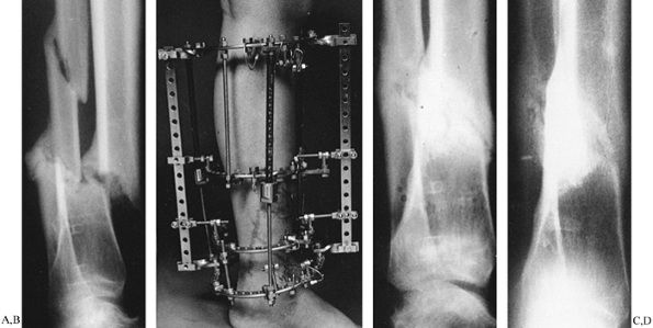 |
|
Figure 32.128. Reduction of a displaced shortened nonunion. A: Eight months after injury. Tibial nonunion with full shaft width displacement and 1 in. of shortening. B: Frame for reduction of displacement and simultaneous lengthening. C: Appearance at the time of fixator removal. D: Appearance at 1-year follow-up.
|
fracture site, there may actually be several nonunions responsible for
the problem. Often, such injuries have been maintained in rigid
external or internal fixation that inhibits osseous healing. When the
fixator is removed, the fracture tends to gradually collapse as the
scar tissue at the site of injury stretches. In some cases, one or more
fracture lines may eventually unite, leaving only one site of retarded
bone healing.
compressing it stimulates osteogenesis. Anecdotal clinical experience
of orthopaedic surgeons in Western countries suggests that bone
formation with this technique is somewhat unpredictable. A more
reliable strategy is to compress the nonunion (either longitudinally or
side-to-side, depending on the obliquity of the fracture line) and
lengthen the bone elsewhere—through healthy tissue—to overcome any
residual limb shortening.
oblique fracture lines are often associated with translation of the
mechanical axis of the distal fragment with respect to that of the
proximal fragment. Not only does such a malalignment retard osseous
healing, but even if the bone did eventually heal in a malaligned
position, the weight-bearing line would fail to pass through the
centers of nearby joints, leading to either chronic joint pain,
degenerative osteoarthritis, or both.
drawing a line through the mechanical axis of each major fragment and
measuring the distance between the lines after correction of angulation
at the nonunion site. Be sure that the roentgenographic projection used
for the measurement shows the displacement at its greatest.
the combined deformity can be eliminated by locating the center of
rotation of the hinge axis at the proper place with respect to the
fragments, as described in the previous section. When displacement
exists without angulation, mutual translation of the fragments is
accomplished by incorporating a translation assembly into the
configuration. The mechanism for a translation assembly is simple yet
elegant: Fix three pairs of horizontal rails to the respective rings
with posts (Fig. 32.129). The entire configuration must be sturdy enough to prevent axial displacement during horizontal translation.
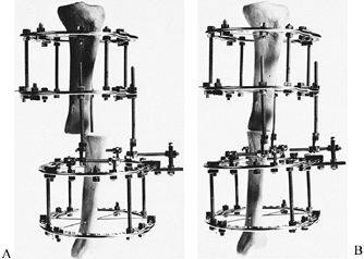 |
|
Figure 32.129. Translation assembly using horizontal rails. A: Before translation. B: After translation.
|
With the Ilizarov method, rotational malalignments are usually corrected last, after angulation, displacement, and shortening (Fig. 32.130).
The reason for this is that the major bone fragments must be aligned
along the same axis to correct malrotation. Moreover, this axis must be
in the center of the configuration. In this way, the bone fragments
will rotate around a line passing through the center of the fixator’s
rings and the marrow canals, rather than through an axis that does not
pass through either. Were the fragments to rotate around an eccentric
axis, one fragment would displace transversely with respect to the
other during rotation.
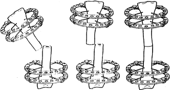 |
|
Figure 32.130. Sequence of correction of rotational malalignment. Angulation is corrected first, and then displacement is addressed.
|
fixation system is the ability to rotate one ring with respect to
another. When unilateral half-pin fixators are used to treat nonunions
and malunions, this capacity for gradual rotational correction does not
exist, no matter how adaptable the fixator may be.
The most stable one uses sliding buckles as the interconnection between
the rotating ring and the rest of the frame. The “motor” that provides
the power to turn one ring with respect to another is made from a
horizontal threaded rod spanning the space between the buckle and a
post connected to the movable ring (Fig. 32.131).
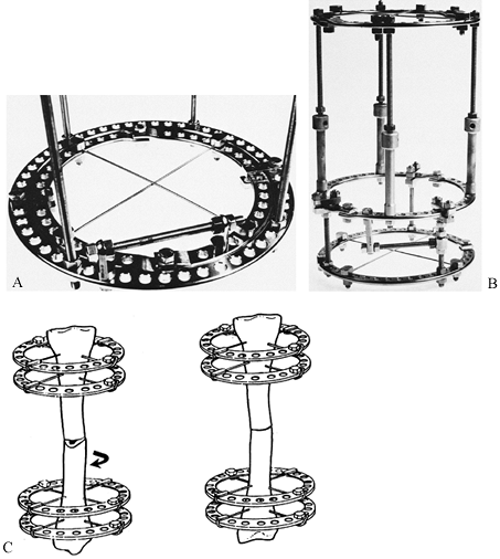 |
|
Figure 32.131. Rotation assemblies. A: Nested rings, with the inner ring securing the wires. B: Buckles-and-bushings rotation assembly. C: The bone fragments must be coaxial—and in the center of the configuration—for counterrotation.
|
threaded rods located between the two rings that must move with respect
to each other. One end of each rod is connected via posts to the upper
ring; the other attaches to posts on the lower ring. Decreasing the
distance between the posts on each rod rotates one ring with respect to
the other.
A pair of clamps made out of two short plates holds the pair of rings
together. In clinical use, the wires are connected to the inner ring
and the fixator to the outer one. A single horizontally oriented
threaded rod attached with posts to each ring will motor the revolution
of the inner ring with respect to the outer one.
and the forearm—the bones are eccentrically placed within the soft
tissues. The tibia, for instance, is anterior and medial in the shank’s
cross section. Placing a fixator around the lower leg would result in a
mounting that rotates around an axis in the soft tissues, rather than
the correct location through the center of the bone. Turning one ring
with respect to another in this situation would cause more displacement
than rotation. For tibial mountings, therefore, a ring for a rotation
assembly must be quite large with the bone—not the leg—centered within
the frame (Fig. 32.132).
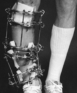 |
|
Figure 32.132. Frame for correction of shortening, malrotation, angulation, and displacement.
|
of trauma, removal of nonviable fragments at initial debridement, or
resection of necrotic bone during the care of an infected fracture.
When a segmental defect is present, any angulation, rotation,
translation, or combination of displacements can easily be corrected
through the soft tissues at the level of the defect. For this reason,
circular frame configurations designed to deal with segmental defects
are usually rather simple: The configuration is tubular, with the
connecting rods of the frame parallel to each other and to the bone’s
mechanical axis.
healthy bone some distance from the defect; then pull the intercalary
segment between the defect and the corticotomy through the tissues
until the defect is closed (1,4,8,12,13,15). At the corticotomy site, new bone forms during distraction (Fig. 32.133).
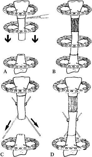 |
|
Figure 32.133. Bone transport diagrams. A,B: Transport with a transport ring. C,D: Transport with oblique directional wires.
|
compressed acutely after appropriate debridement, and the bone can be
lengthened through a corticotomy elsewhere.
more than 2.5 cm, since the redundant soft tissues surrounding the
defect tend to bulge when the fragments are brought together, creating
an unsightly appearance to the leg and kinking both lymphatic and
venous drainage. As this redundant skin is trapped between the wires,
it cannot contribute to lengthening of the limb through another section
of the bone. Therefore, the patient is left with a peculiar-looking
limb with bulky redundant tissues at one level and tight, stretched
skin at another. With this problem in mind, when dealing with a
segmental defect of more than 2.5 cm, leave the soft tissues at length
and eliminate the defect by gradual transport of the intermediate
segment.
transport ring and cross-wires, or with oblique directional wires. A
transport ring and an attached pair of cross-wires is the most stable
way to pull a bone fragment through
tissue (Fig. 32.134).
Unfortunately, the wires must cut through the skin and soft tissues as
the ring and its attached bone segment move through the limb. At the
end of bone transport, however, the crossed wires serve to enhance
compression at the point of contact between the intermediate fragment
and the target fragment.
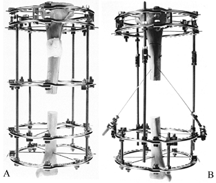 |
|
Figure 32.134. Bone transport frames. A: Transport with a transport ring. B: Transport with oblique directional wires.
|
segment through a limb, there is far less cutting of tissues, since the
wires start out nearly parallel to the limb’s axis (Fig. 32.134).
Unfortunately, such oblique wires often do not provide enough pressure
at the end of bone transport to ensure stable interfragmentary
compression between the intermediate fragment and the target fragment.
For this reason, a pair of cross-wires connected to a ring must be
attached to the intermediate fragment at the end of bone transport to
enhance compression at the point of contact. In such a case, a second
operation is required.
through the limb, it is obvious that the proximal fragment, the
intermediate fragment, and the distal fragment must all be in line with
each other lest the intercalary fragment miss its target. Although such
a requirement seems simple, in actual practice the bone fragments tend
to sag posteriorly on the operating table while a frame is being
applied. Be sure to check the final alignment of the bone fragments on
long x-ray films before the patient leaves the operating table.
afterwards, this is not preferred. A fragment of bone can be moved
within its ring by detaching the transfixion wires from their fixation
bolts and moving the wires over one or two holes on the ring.
for a skeletal defect deals with the shape of the bone ends at the
docking site (Fig. 32.135). Unfortunately, it
is difficult to match bone ends on opposite sides of a skeletal defect
so that they fit well together when a defect is closed. The most
predictable healing occurs when one fragment impales the marrow cavity
of the other (Fig. 32.136). Of course, the
surgeon must trim a point on the transported segment for such
impalement to be possible. Regardless of the shape of the bone ends, we
do not hesitate to insert a bone graft around the contact point between
the transported and the target fragments whenever we suspect that
healing will be delayed.
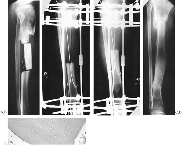 |
|
Figure 32.135. Bone transport case requiring a small bone graft at the docking site. A:
Initial condition. A block of methylmethacrylate is used as a spacer in the mid tibia. Multiple sinus tracts are present, draining pus. B: After removal of spacer and resection of nonviable bone. C: During bone transport with directional wires. D: A nonunion is noted at the docking site at the time of fixator removal. E: Biopsy demonstrating nonviable bone at the end of the intercalary fragment. |
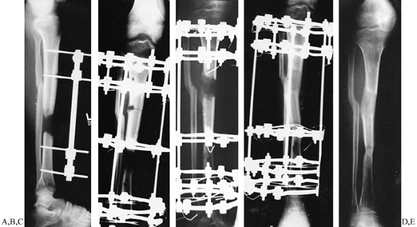 |
|
Figure 32.136.
Bone transport case with impalement of intercalary segment into target segment. The patient also has a cavity osteomyelitis caused by a pin. A: Initial condition, showing osteolysis around lower pin in proximal fragment. B: Radiograph at time of fixator application and corticotomy through the pin site. C: Radiograph at 6 weeks of distraction. D: Radiograph at end of distraction. E: Final appearance. No bone graft was needed. |
shortening. In many cases, simply stretching the defect will restore
limb length. When a limb segment contains but a single
bone,
such as the humerus or the femur, shortening is eliminated either at
the time the fixator is applied (by stretching the soft tissues of the
defect to full length) or by lengthening through the corticotomy site
after the intermediate fragment has completed its journey.
with a segmental defect, elongation after bone transport can occur only
if there is a nonunion or osteotomy through the other bone in the limb
segment. With an intact parallel bone, perform osteotomy of the intact
bone at the same time as the corticotomy of the bone with the defect.
Thereafter, both the corticotomy site of the bone with the defect and
the osteotomy site of the intact bone are lengthened simultaneously (Fig. 32.137). When the limb is at full length, continue transport of the bone with the defect until the defect is eliminated.
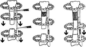 |
|
Figure 32.137.
Bone transport with shortening. The fibular and tibial corticotomies are made at the same time, and the limb is lengthened before bone transport. |
ways simpler than managing a nonunion, yet in other ways it is more
challenging. For instance, with a nonunion, it is usually possible to
correct the deformity through the nonunion site. In correcting
malunions, another option is to osteotomize the bone at a site away
from the fracture deformity. In this manner, both dense corticalized
fracture callus and damaged soft tissues at the fracture site are
avoided. On the other hand, correcting a malaligned limb through a
location that does not correspond to the apex of the true deformity may
leave the patient with an ugly hump on the limb after the bone’s axis
is restored. For this reason, choose the osteotomy site carefully, with
due consideration for the quality of bone available, the need for
lengthening, and cosmesis (14).
two levels. In these cases, corrective osteotomies must often be
performed near both malunions. Most posttraumatic malunions result in
limb shortening. Sometimes the
shortening
is a relatively straightforward matter: Simply unfolding an angulated
malunion through its apex will restore length. In such patients, the
loss of length is caused by the angulation. In other cases, realignment
of the fragments fails to overcome loss of length.
and shortening, but also translation (displacement) of the mechanical
axes of the fragments, and rotation as well. Sometimes these
deformities are not as apparent as angulation and shortening, but,
unless the surgeon is aware of associated malalignments, the correction
will be less than ideal.
angulation, follow the recommendations in the above section on
angulated nonunions.
translation, or some other combination of factors resulting in both
angulation and true shortening of the bone, correcting the angulation
and realigning the bone’s mechanical axis will not result in
restoration of limb length without using a distractional hinge or a
translation hinge, or lengthening after deformity correction.
consistent malunion deformities. For example, a distal tibial fracture
with associated fracture of the fibula that has healed in a shortened
position and angulated into valgus usually demonstrates external
rotation of the distal tibial fragment and foot and lateral
displacement of the distal fragment’s mechanical axis compared to that
of a proximal fragment. Malunions with varus of the tibia frequently
are rotated inward and displaced medially.
intersection of the mechanical axes of the principal fragments. In
angulated malunions without concomitant displacement, the intersection
point is at the level of the old fracture line. When displacement
accompanies angulation, the intersection of the axes of the fragments
is not at the fracture line, but at some point above or below the level
of injury. Placing a corrective osteotomy at the level of the apex of
the deformity corrects angulation of the fragments but does not improve
translation of their mechanical axes. To correct such displacement, the
cortical osteotomy must be level proximal or distal to the hinge axis
at the apex of the deformity. When the level of the corticotomy and
hinge axis of the configuration are not at the same level, correcting
angulation automatically results in translation of the bone fragments.
The geometry of correction in this manner was described earlier in this
chapter by Paley and Tetsworth.
in separate steps, using a fixator configuration that incorporates
assemblies for both angular correction and translation. Such frames are
fairly complicated, since the translation mechanism involves multiple
horizontal threaded rods connected to adjacent rings on both sides of
the apparatus.
other deformities—must be corrected with an assembly that permits the
corresponding rings to rotate with respect to each other. As a general
principle, begin counterrotation of fragments after correction of
angulation and restoration of limb length. In many situations,
correction of displacement can accompany rotation, especially if the
mechanical axes of the major bone fragments are not located within the
center of their corresponding rings.
the various deformities that require correction, make cutouts of the
bone segments and perform the surgery with paper and tape before the
actual operation.
roentgenograms of lower-extremity problems and corresponding films for
upper-limb malunions. Also obtain roentgenograms of both the involved
and normal bones in multiple projections, one of which shows the
maximum deformity in profile, the view perpendicular to the true plane
of the deformity. If there are two or more deformities in the bone that
are oriented in different planes, then obtain separate roentgenographic
projections of each deformity in its maximum profile. With long tracing
paper, make cutouts of the abnormal bone and perform the osteotomies at
appropriate levels to correct the deformity. In complex cases, make the
tracings on large clear acetate sheets, using separate pieces for the
proximal and distal fragments. In this way, the traced fragments can be
rotated with respect to each other, using a thumbtack as the hinge
axis. Moving the thumbtack around in different locations outside the
contours of the fragments will often reveal the correct location of the
point of rotation for correction of both angulation and displacement.
follows the principles of general deformity correction with the
Ilizarov method.
spinal mechanics, may require ungainly shoe lifts, and often
embarrasses the patient. Before the introduction of the Ilizarov
methods, a posttraumatic leg-length discrepancy in an adult was usually
managed with either a shoe lift, shortening the contralateral limb, or
in rare instances lengthening with an open osteotomy and multiple
surgeries. The
discovery
of bone’s capacity to regenerate in a widening distraction gap has
revolutionized the care of posttraumatic limb-length inequality (14).
fewer problems than elongating a congenitally short limb, for the
following reasons. First, before injury, the neurovascular structures
were at full length; with elongation, these structures are restored to
their original status. Second, posttraumatic shortening usually
involves a loss of length of 3–7 cm, whereas congenitally short limbs
often demonstrate far greater inequality. Third, the skin and soft
tissues are often redundant after posttraumatic shortening and
therefore easy to lengthen.
posttraumatic shortening may present significant problems, especially
if there is extensive scar tissue, preexisting microvascular repair,
transposition flap surgery, or injury to neurovascular structures,
muscles, or tendons. Also, damaged joints, internal fixation devices,
disuse osteoporosis, articular contractures, head trauma, and other
problems may complicate restoration of limb length for posttraumatic
shortening.
limb follows the same methods used for limb elongation associated with
other kinds of pathology. Apply a stable external skeletal fixator and
perform a corticotomy through healthy bone surrounded by normal soft
tissues (2,3,5).
After a delay of 5–7 days, lengthen the limb using Ilizarov’s
guidelines. If the soft tissues around the corticotomy level are
suboptimal, prolong the latency up to 14 days.
divided doses. Manage any delay of new bone formation in the
distraction gap by slowing the rate of distraction to 0.5–0.75 mm per
day (a distraction frequency of 0.25 mm every 8–12 hr). Concomitant
deformities must be corrected during lengthening following the
principles described in preceding sections.
limb-lengthening program. Treat any joint that develops a contracture
vigorously. Progression of a flexion contracture of the knee, for
example, can lead first to posterior subluxation of the tibia on the
femur, and then to frank dislocation of the knee joint. Likewise,
lengthening a femur with either a valgus hip deformity or a shallow
acetabular roof can lead to subluxation or dislocation of the hip.
elongation (or deformity correction, or any other application of an
external fixator) must be investigated and corrected. Often, pin or
wire site sepsis is the problem. Muscle impalement or pain caused by
irritation of tendons or synovium also interferes with gait.
Contractures limit ambulation. Decreased weight-bearing leads to
osteoporosis, a cause of pin or wire loosening. The loosened implants
lead to fixator instability, which causes further pain and infections.
This vicious cycle must be stopped as soon as it appears. Check for
fixator stability and range of joint motion at each visit. Ask the
patient about pain and any reasons for a decline in the ability to
walk. If necessary, admit the patient to the hospital for intensive
physiotherapy (primarily muscle stretching). Stop the lengthening for a
week if necessary. Change any infected pins or wires if sepsis cannot
be controlled with antibiotics.
lengthening. Instead, stop or even back up a bit and allow the bone to
mature. Six or 8 months later, when joint function has been restored to
normal and the patient is fully ambulatory, repeat the lengthening.
scheme: *, classic article; #, review article; !, basic research
article; and +, clinical results/outcome study.
GA. The Tension-Stress Effect on the Genesis and Growth of Tissues:
Part I. The Influence of Stability of Fixation and Soft-Tissue
Preservation. Clin Orthop 1989;238:249.
GA. The Tension-Stress Effect on the Genesis and Growth of Tissues:
Part II. The Influence of the Rate and Frequency of Distraction. Clin Orthop 1989;239:263.
GA. Angular Deformities with Shortening. In: Coombs R, Green S,
Sarmiento A, eds. External Fixation and Functional Bracing. Frederick,
MD: Aspen, 1989.
GA. Fractures and Nonunions. In: Coombs R, Green S, Sarmiento A, eds.
External Fixation and Functional Bracing. Frederick, MD: Aspen, 1989.